Categories
Offsites

Quantified Self Part 6 – 생산적인 하루에 대한 정량적인 표현과 4년간의 데이터 이야기

이번 포스트에서는 그 동안 모아온 데이터에 대한 이야기를 집중적으로 해보려고 합니다. 왜 이 데이터들을 모았는지, 그리고 그 동안 모아온 데이터가 무엇을 말하고 있는지에 대한 이야기 입니다.

images

출처 : http://quantifiedself.com/

지금까지의 시리즈

Github: https://github.com/DongjunLee/quantified-self

‘오늘 하루 알차게 보냈다!’ 이 말을 숫자로 표현할 수 있을까요?

Quantified Self 를 주제로 사이드 프로젝트를 진행하면서, 정량적으로 정의하고 싶던 것이 있습니다.
‘오늘 하루 알차게 보냈다!, 뿌듯하다!’ 혹은 ‘아.. 오늘은 아무것도 한 것이 없네..’ 이러한 하루하루에 대한 느낌들 입니다. 느낌이라는 것 자체가 주관적이라는 것을 알고 계실 것입니다. 하루에 대한 평가는 주관이 기본이 되며, 특히 개개인이 가지는 가치관 이라던가, 선호에 따라서 각각 다르게 평가할 수 있습니다. 그래서 실 데이터를 보면서 오늘 하루를 제가 어떤 식으로 평가를 할 것인지 이야기하기 전에, 제가 중요하게 여기는 것을 먼저 이야기 해보고자 합니다.

저는 ‘습관’을 굉장히 중요시 여기고, 하루하루 무언가 꾸준히 하면서 쌓아올린 것이 결국에 나중에 결과를 만들어 낸다고 믿고 있습니다. 이 칼럼(습관은 자신의 참 모습을 보여주는 창이다)에서, 제가 생각하는 습관의 중요성을 잘 말해주고 있습니다.

계몽주의 철학자 데이비드 흄은 이런 습관에 대한 고대와 중세의 해석을 더욱 확장했습니다. 흄은 습관이 바로 인간을 인간으로 만든다고 생각했습니다. 그는 습관을 모든 ‘정신이 그 작동을 의지’하는, ’우주의 접착제(cement)’라 불렀습니다. 예를 들어, 우리는 공을 높이 던지고 떨어지는 것을 볼 수 있습니다. 그는 습관에 의해 우리가 몸을 움직여 공을 던지고 그 공의 궤적을 바라볼 수 있으며, 이를 통해 원인과 결과의 관계를 파악할 수 있다고 생각했습니다. 흄에게 인과론은 바로 습관에 의한 연상작용이었습니다. 그는 언어, 음악, 인간관계 등 경험을 유용한 무언가로 바꾸는 모든 기술이 습관에 의해 만들어진다고 믿었습니다. 곧, 습관은 우리가 세상을 살아가고 이 세상의 원리를 이해하기 위해 반드시 필요한 도구였습니다. 흄에게 습관은 ‘인간 삶의 거대한 안내자’였습니다.

습관에서 ‘무엇을 할 것인가’ 역시 굉장히 중요한 주제입니다. 여기에는 당장 해야 하는 일 보다는 자기 계발에 해당하는 일들이 해당됩니다.
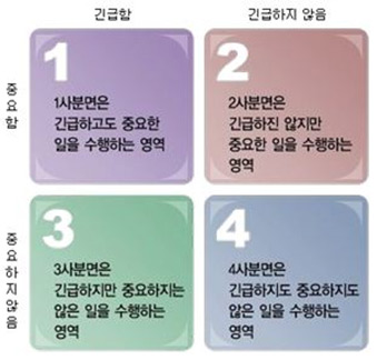
image.png

스티븐 코비의 시간관리 매트릭스

작업에는 몇가지 종류가 있습니다. <성공하는 사람들의 7가지 습관> 에서 나오는 시간관리 매트릭스가 그 중의 하나 일 것 입니다. ‘긴급함’ 과 ‘중요함’ 2가지 척도로서 작업들을 나누는 것입니다. 여기서 제 2사분면은 중장기 계획, 인간관계 유지, 자기계발 등 당장 급하지는 않지만 미래에 큰 보상을 주는 일들이 포함됩니다.

목표는 이렇게 정리할 수 있겠네요.

  1. 자신이 발전할 수 있는 일들에 시간을 많이 사용하고,
  2. 이 활동들을 꾸준히 지속하는 것

이제 제가 어떠한 하루들을 목표로 하는 지 이해 하셨을 것이라 생각이 됩니다. 그 동안의 포스트에서는 데이터를 수집하기 위한 준비와, 그 과정에서 몇가지 자동화도 작업 해보았습니다. 최근 포스트에서는 데이터 시각화도 하면서 대쉬보드도 만들어보았지요. 이 일련의 작업들의 궁극적인 목적은 실제 데이터들을 보면서, ‘생산적인 하루’를 보내고 있는지, 이런 하루를 보내려면 앞으로 어떻게 하면 좋을지 데이터를 보면서 저 자신을 더 깊게 이해하기 위함이였습니다.

생산적인 하루에 대한 Metric 을 정해보자.

생산적인 하루를 정량적인 숫자로 표현하기 위해서는 몇가지 단계를 거칠 필요가 있습니다. ‘오늘 하루 알차게 보냈다!’ 이 문장을 분해를 하는 것입니다. 먼저 이 느낌에 포함이 되는 요소들은 무엇이 있을까요? 예를 들어, 이런 요소들이 있을 것 입니다. 잠은 잘 잤는지, 하려고 했던 To do list 는 다 완료 했는지, 또 그 작업들을 할때 집중해서 했는지, 하루를 기분 좋게 보냈는지, 크게는 이러한 요소들이 있을 것 입니다.

제가 뽑은 요소는 다음의 5가지 입니다. Attention, Happy, Productive, Sleep, Habit. 이제 각각의 요소들을 어떻게 정량적으로 평가할 수 있을지 한번 더 단계를 들어가서 보시죠.

Attention, 작업에 대한 집중

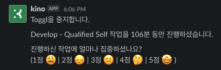
  • 진행한 작업들에 대해서 얼마나 집중했는지는 의미합니다.
  • 기본적으로 40분 이상 진행한 작업에 대해서 집중도를 물어보게 만들어 놓았습니다.
  • 집중도에 대한 점수는 1~5점 척도로 되어있습니다.
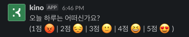
image.png

Happy, 그 당시의 기분

  • 하루를 기준으로 200분 마다 그 당시의 기분에 대해서 물어봅니다.
  • 행복도에 대한 점수 역시 1~5점이 기준입니다.

image.png

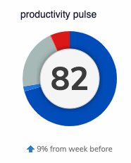
Productive, 각종 Tool을 활용한 생산성 점수

  • RescueTime 는 PC/모바일을 사용한 기록을 가지고 Productive Pulse 라는 점수를 계산하여 제공해주고 있습니다. (이 값이 어떻게 구해지는 지는 이 링크에서 확인하실 수 있습니다.)

image.png

  • Toggl 에서는 오늘 하루 기록된 작업시간이 8시간 이상부터 100점, 그 아래로는 시간에 비례해서 점수를 차감합니다.
    (예를 들어, 7시간 작업 시 → 87.5점, 6시간 작업 시 → 75점)

image.png

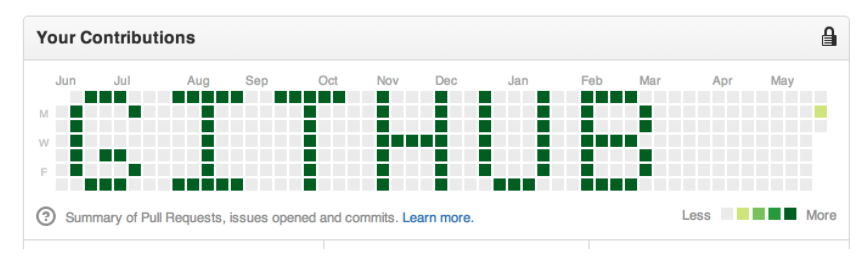
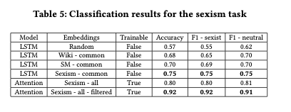
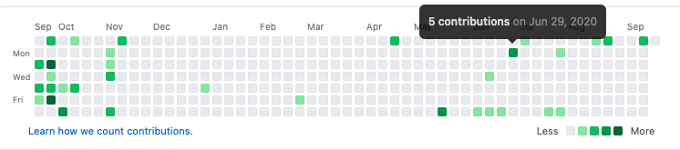
  • Github 에서 오늘을 기준으로 10일 동안의 Commit의 합이 10개 이상부터 100점, 그 아래로는 커밋 수에 비례해서 측정됩니다. 아래 contributions 의 수를 의미합니다.

image.png

  • Todoist 에서는 100점을 기준으로, 완료하지 못한 일들 (+ 기한이 지난 경우 포함)을 우선순위에 따라 차감을 하게 됩니다.
    우선순위는 아래와 같이 4가지가 있고, 높은 우선 순위부터 5, 4, 3, 2 점씩 차감이 됩니다.

image.png

  • 위의 각각의 항목들은 모두 100점 만점이 기준이 됩니다. 여기서 종합 생산성 점수는 다음과 같습니다

Productive = Github (10) + Toggl (30) + Todoist (50) + RescueTime (10)

Sleep, 수면 시간

  • 7시간을 이상은 전부 100점, 그 아래로는 시간과 비례해서 점수를 측정합니다.
  • 수면에 대해서는 약간 관대하게 점수를 재고 있었습니다. (너무 잠을 많이 자는 것이 오히려 피곤함을 초래하는 경우도 있기 때문이죠)

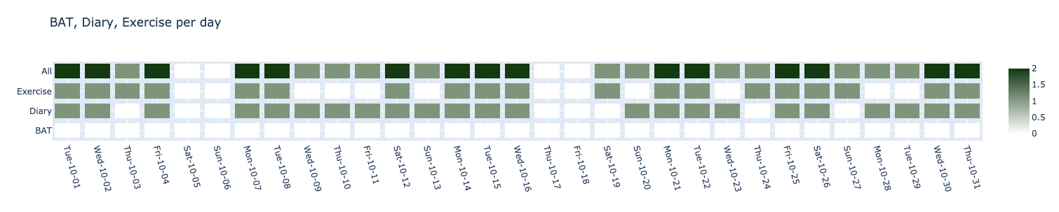
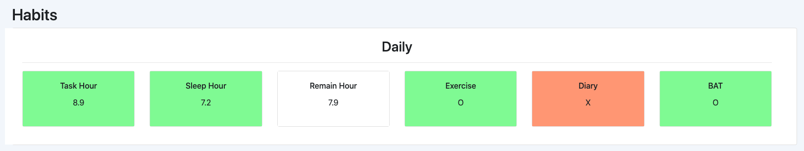
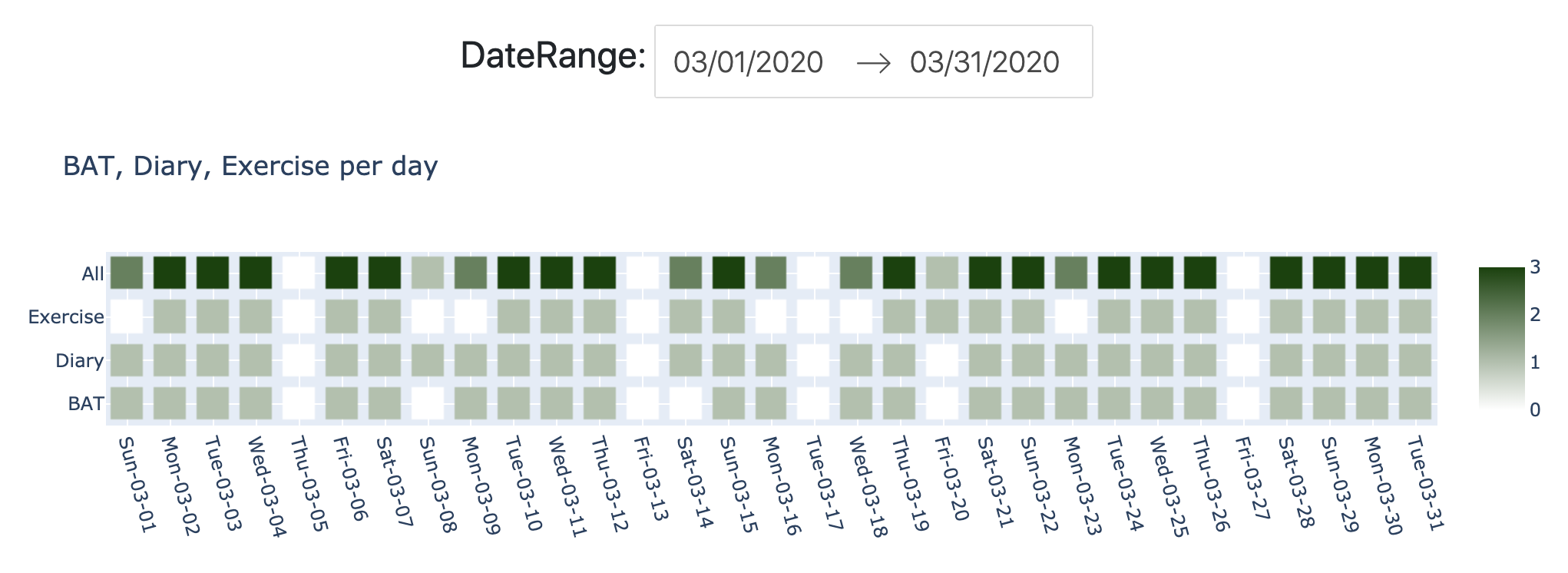
Habit, 매일하는 습관에 해당하는 활동들

  • 개별 항목 하나하나가 5점의 점수를 가집니다.
  • 매일 하려고 하는 습관에 해당하는 일로서 다음의 일들이 습관에 해당합니다.
    • 운동
    • 공부한 것 정리
    • 일기

이제 각각의 항목들을 정리했으니, 마지막으로 이 각각의 점수를 종합해서 오늘 하루를 점수를 매겨보겠습니다.

오늘 하루에 대한 점수 = Attention(20) + Happy(10) + Productive(30) + Sleep(20) + RepeatTask(10) + Habit(15)

이 기준을 모두 만족하면서, 100점을 얻으려면 다음과 같은 일들이 필요합니다. 모든 진행한 작업들에 대해서 집중을 해야하고, 기분도 좋아야 하며, 일일커밋 역시 꾸준히 해주고, 8시간 이상 생산적인 작업을 하고, 등록했던 모든 To do list는 완료를 하고, 컴퓨터를 생산적인 소스 위주로 작업을 하면서, 잠은 7시간 이상 자고, 운동, 공부한 것 정리, 일기 모두 완료를 해야겠네요….😱

이렇게 제가 바라보는 오늘 하루에 대한 점수를 정량화 할 수 있는 식을 만들어 보았습니다. 처음 말한 것처럼, 무엇을 중요시하는 지에 따라서 점수에 대한 비중은 조절할 수 있을 것이고 자신의 생활 패턴에 따라서 기록할 수 있는 수단 또한 달라 질 수 있을 것 입니다.

4년 간의 데이터가 말해주는 것들

사이드 프로젝트를 시작하고, 데이터를 수집하기 시작한 것은 2017-01-30 부터 입니다. 대략 4년째 이렇게 계속해서 Kino를 사용하고 있습니다. 특별히 문제가 없는 이상, 앞으로도 이렇게 사용을 하게 될 것 같네요. 🙂

그럼 그 동안의 데이터의 변화를 보면서 제가 생산적인 하루들을 보냈는지 이야기 해보려고 합니다.

image.png

그림 1 – 월간 종합점수의 변화

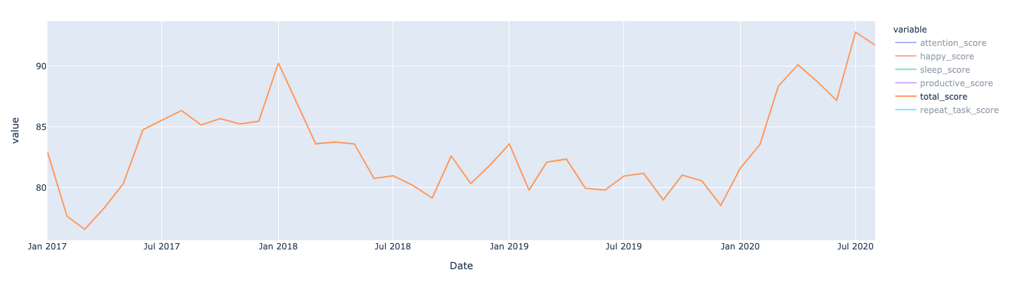
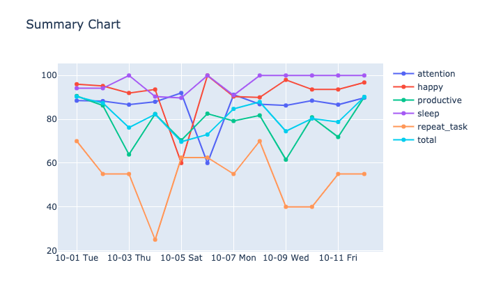
위의 도표는 월간 평균 total_score(종합 점수) 를 기준으로 만들어진 라인 차트입니다. 사이드 프로젝트를 시작하는 초반에 열심히 하면서 점수가 올라가다가.. 2018년 상반기부터 떨어지기 시작하는 것이 보입니다. 이 시기가 네이버로 이직을 했던 시기인데, 이직을 하고 나서는 사이드 프로젝트 및 따로 진행했던 ML/DL 논문 구현 들은 하지 않고 회사 일에 더 집중했던 시기입니다. 그리고 2020년부터는 다시 이 QS 프로젝트에 신경을 쓰면서 점수가 올라간 시기입니다. 회사 일도 좋지만, 그 외의 시간을 잘 활용하는 것이 중요한 것 같다는 생각이 드네요. 조금 더 자세히 데이터들을 살펴보려고 합니다.

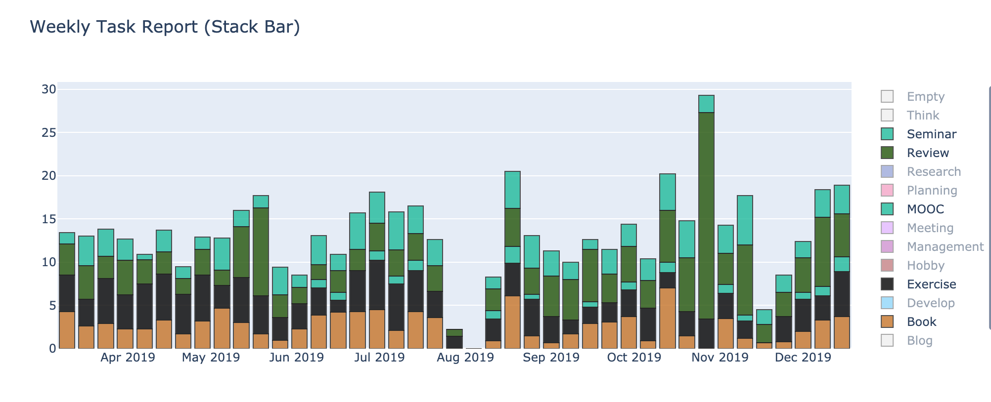
사이드 프로젝트의 재미 그리고 연구/개발에서 미팅/관리 작업으로

image.png

그림 2 – 각각의 월을 기준으로 각 작업들의 작업시간을 카테고리에 따라 누적한 누적막대차트

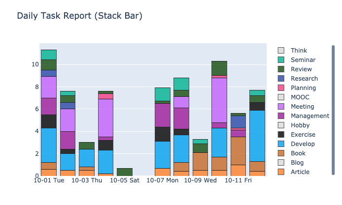
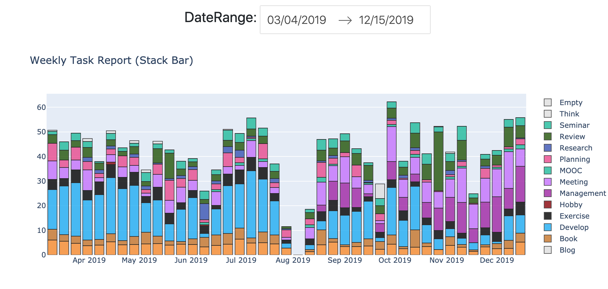
이 도표는 월을 기준으로, 각 작업들의 시간을 누적막대로 구성하였습니다. 주요한 작업들인 연구/개발과 미팅/관리만을 표시해보았습니다. 위에서 언급한 것처럼, 2017년에는 이 QS 사이드 프로젝트를 정말 재미있게 개발을 하던 시기이기도 하고, Deep Learning 공부를 하면서 논문 재구현에 힘을 쓰던 시기이기도 합니다. 실제로 작업 시간의 차이가 유의미하게 크기 때문에.. 종합 점수의 차이 또한 이해가 되네요.
2019년도에는 미팅/관리의 작업들이 확 늘어나게 되는데, 커리어의 변화가 이렇게 보이기도 합니다. 관련해서 커리에 대한 이야기는 2019 회고에서 더 자세히 확인할 수 있습니다.

생산적인 하루에 대한 상관관계

이제 다음 데이터를 조금 더 자세히 살펴볼까요? 먼저 보고자 하는 것은 잠 입니다.
‘잠을 더 자면, 그 날의 기분이 더 좋을 것인가?’ 라는 직관적인 생각을 확인해보고자 합니다.

image.png

그림 3- 수면시간에 따른 행복도 점수의 산점도 차트

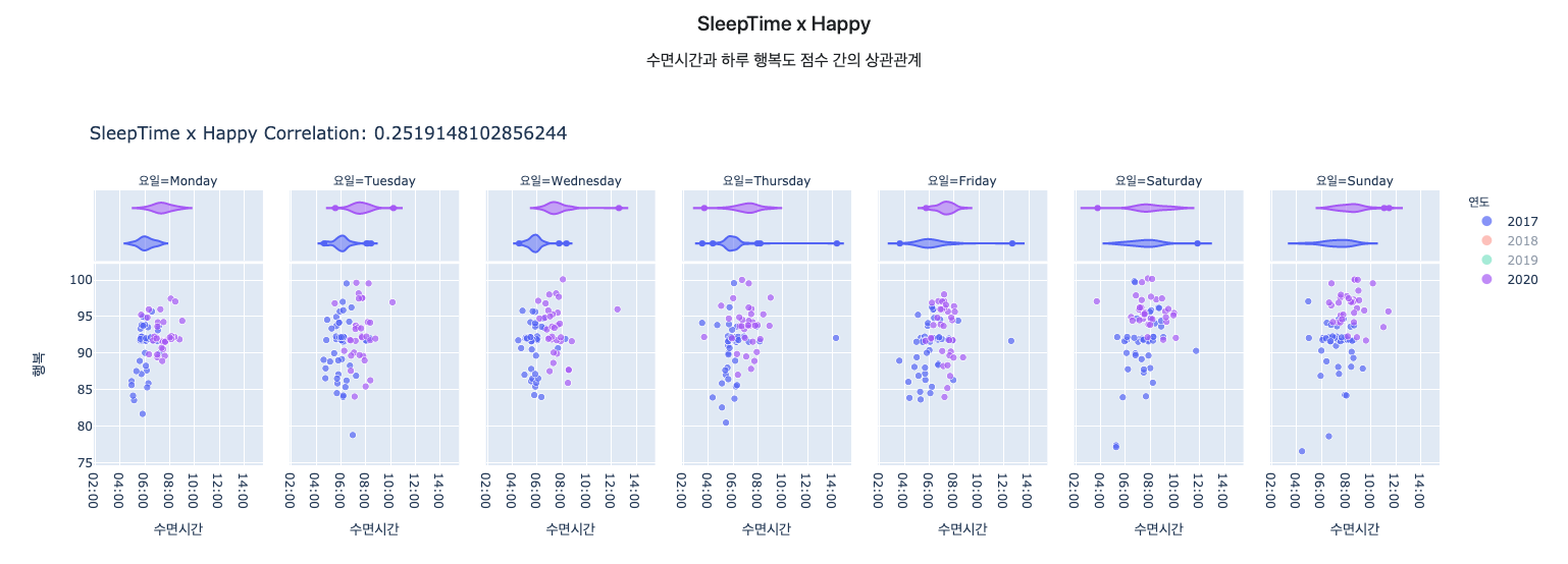
위 도표를 보면 2017년도의 점들이 2020년에 비해서 왼쪽에 위치한 경향성을 확인할 수 있습니다. 2017년에는 평일에는 보통 5~6시간을 잤고, 2020년에 7~8시간을 자는 것을 확인할 수 있습니다. 이것은 사실 통근 시간에 따른 삶의 질을 확연하게 보여주는 것이기도 합니다. 각각의 연도에 집에서 회사까지 출근하는 시간이 각각 1시간 30분, 30분 이 걸리기 때문이죠. (이렇게 통근 시간이 중요합니다..)

수면 시간은 여러가지로 생활에 영향을 미칠 것 입니다. 예전에 왕복 3시간 통근 하던 때를 추억해보면, 아주 큰 영향이라고 느껴집니다. 데이터는 어떻게 말을 해줄까요? 수면시간과 하루의 행복도 점수 평균에 대한 상관 계수 (0.252) 로 약한 상관관계가 있다는 것을 알 수가 있습니다. 제가 느끼는 느낌의 정도와 상관계수는 차이가 있어보이나, 수면시간의 중요성은 똑같이 말을 해주고 있습니다.

다음으로 종합 점수에 대해서 전체 상관관계를 한번 봐볼까요?

image.png

그림 4 – 수면시간, 작업 수와 작업시간, 그리고 각종 점수들의 상관계수

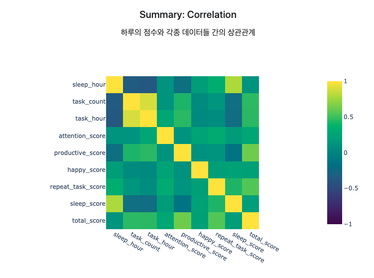
종합점수에 대해서 가장 강한 상관관계를 가지고 있는 것은 ‘생산성 점수’ (0.62) 입니다. 종합 점수에서 30%으로 가장 큰 비율을 차지하고 있기도 하고, 생산성 점수와 작업의 집중도는 연결되어 있기 때문에 어쩌면 당연한 결과일 것 입니다. 그 다음으로는 점수의 변동이 큰 반복작업 점수 (0.54), 작업시간 (0.42) 으로 작업에 관한 것들이 또한 강한 상관관계를 보여주고 있습니다. 수면 점수(0.20) 와 행복도 점수(0.22) 그리고 집중도 점수(0.27) 는 상대적으로 약한 상관 관계를 보여주고 있네요. 지금의 Metric에서의 생산성은 일정한 기준을 통과하면 만점을 주고 있기 때문에, 질보다는 기본적인 양이 더 중요하게 고려되고 있음을 말해주고 있습니다.

상관계수를 보다 보니, 막연하게 알고 있던 것을 데이터를 통해 확인할 수 있었습니다. 바로 잠을 포기하고 작업을 하는 경우 입니다. 수면시간과 작업시간 간의 상관계수는 (-0.37)으로 음의 상관관계를 보여주고 있습니다. 그에 비해서 수면시간과 집중도 간의 상관계수는 (0.11)으로 아주 약한 상관관계를 보이고 있습니다. 직관적으로는 수면시간이 작업 집중도에 중요한 요소일 것이라고 생각하였는데, 생각과는 약간 다른 결과를 보여주고 있네요. 오히려 수면 시간 보다는 그날의 기분 (0.25) 가 더 상관계수가 높았습니다. 위에서 수면시간과 행복도에 대한 약한 상관관계가 있음을 확인했었기 때문에, 같이 연결해서 봐야할 것입니다.

여기서 지금 Metric의 한계점이 보이기도 합니다. 잠을 줄이면서 공부를 더 한다면, 평소보다 점수는 더 높게 나올 것 입니다. 하지만 ‘꾸준함’을 생각해보면 잠 또한 더 중요하게 생각해야 할 것입니다. 이런 한계점들에 대해서는 아래에서 더 나은 Metric 에서 이야기를 해보고자 합니다.

다음으로는 종합점수와 가장 높은 상관 관계를 보이는 작업에 대해서 조금 더 디테일하게 살펴보겠습니다.

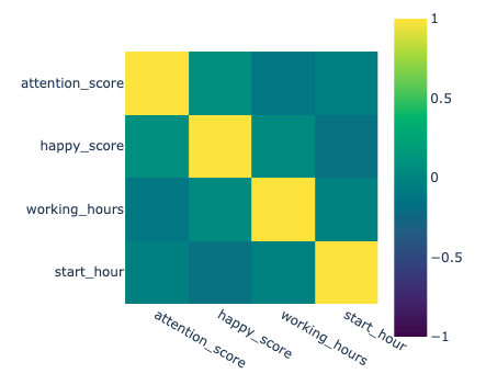
작업의 종류에 따른 집중도와 각 변수들과의 상관계수

어떠한 작업에 대해서 집중도에 관여하는 요소들은 무엇이 있을까요? (Category) 어떠한 작업을 하는지, (When) 언제 하는지, (Mood) 그 당시의 기분은 어떠한지, 조금 더 세부적으로 들어가면 방해요소는 없었는지, 난이도는 적절한지 등의 다양한 요소가 있을 것 입니다. 여기서 데이터를 보려고 하는 것은 작업의 종류, 시간대, 기분을 가지고 살펴보려고 합니다.

여기에는 아래와 같은 가정을 가지고 살펴보려고 합니다.

  • 일에 더 집중하게 될 수록, 그에 따라서 기분도 좋다.
    (몰입, 집중도 점수와 행복도 점수의 상관관계가 높은 경우)
  • 작업을 오래 할수록, 해당 작업에 집중할 수도 있고 집중이 안 될 수도 있다.
    (집중도 점수와 작업시간의 상관관계)
  • 작업은 언제 시작하느냐에 따라서 집중도에 영향을 줄 수 있다.
    (집중도 점수와 시작시간의 상관관계)
    예) 12시에 점심식사 시간인데, 11시 반에 개발을 시작하는 경우

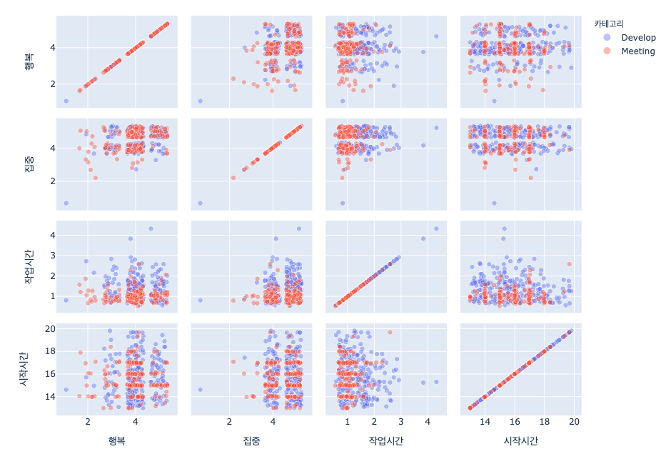
지금처럼 고려되는 범주의 수가 3개 이상일 때는 산점도 매트릭스가 범주 간의 관계를 확인할 수 있어서 적합한 방식입니다.

image.png

그림 5-1 평일 오전 시간대(오전 10시 ~ 오후 1시)의 ‘개발’, ‘미팅’ 에 대한 산점도 매트릭스

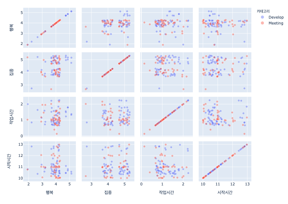
작업은 굉장히 다양한 조건들이 있기 때문에, 세부적으로 조건을 가지고 살펴볼 필요가 있습니다. 위 도표는 오전시간을 대상으로 ‘개발’, ‘미팅’ 에 대한 산점도 매트릭스 입니다. 눈으로 확인할 수 있는 작업의 특성은 다음과 같습니다. 미팅은 보통 1시간 단위로 진행이 되므로 10, 11, 12 시에 몰려있는 것을 알 수가 있습니다. 그리고 개발에 대한 작업은 최소 1시간 정도의 집중을 위한 시간을 필요로 하기 때문에, 10시~11시 사이에 밀집되어 있는 것을 확인할 수 있습니다. 이러한 현상을 상관계수로도 확인을 할 수가 있습니다.

image.png

그림 5-2 평일 오전 시간의 ‘개발’, ‘미팅’ 에 대한 상관계수

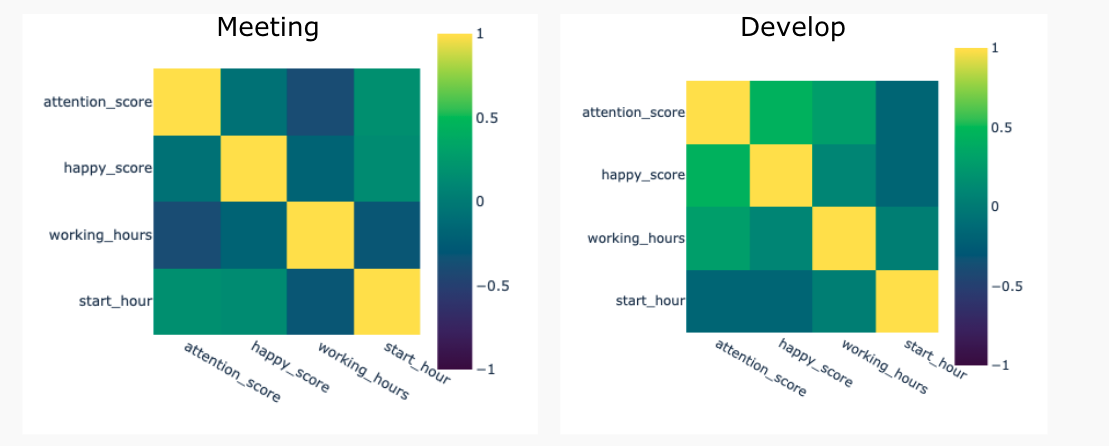
위의 상관계수 도표를 통해서, 집중도와 각 변수들간의 관계가 차이가 있음이 눈에 확인히 보입니다. 눈에 띄는 차이는 1) 행복도점수와 2) 작업 시간 입니다.

먼저 행복점수 입니다. 개발을 하면서 일에 집중하면 할수록, 그에 따라서 기분이 좋음(0.44)을 보이고 있습니다. 그에 비해서 미팅의 경우에는 작업과 행복도 간에는 상관관계가 없다(-0.07)고 볼 수 있습니다. 오전에는 미팅보다는 개발 작업을 하는 것이 더욱 집중하면서 진행한다는 것을 말해주고 있지 않나 싶습니다.

다음은 작업 시간입니다. 위에서 말한 것과 비슷한 경향으로서, 오전에 진행하는 미팅의 경우 시간이 길수록 집중력이 떨어지는 경향(-0.39)이 보이는 반면 개발은 작업시간이 길수록 더 집중력이 높았던 경향(0.29)을 보이고 있습니다.

image.png

그림 6-1 평일 오후 시간대 (오후 1~8시)의 ‘개발’, ‘미팅’ 에 대한 산점도 매트릭스

위의 도표는 오후 시간대에 대한 같은 조건의 산점도 매트릭스입니다. 오전보다는 오후 시간을 더 길게 활용하고 있기 때문에 점들이 확실히 더 많아 보이네요. 여기에서도 오전에서와 비슷하게, 미팅작업은 대부분 정시에 몰려있는 모습이 보이고, 미팅은 보통 1시간, 개발은 1~2시 사이에 몰려있는 것을 확인할 수 있습니다. 그리고 개발에서는 대부분 행복도 점수가 3~5 점이나, 미팅 작업에서 행복도 점수가 2점으로 떨어진 경우들도 보입니다. 이것은 개발에 비해서 상대적으로 컨트롤이 어려운, 미팅이 가지는 특성이 아닐까 싶습니다.

image.png

그림 6-2 평일 오후 시간의 ‘개발’, ‘미팅’ 에 대한 상관계수

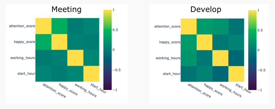
오전과 마찬가지로 상관계수를 살펴보겠습니다. 위와 마찬가지로 1) 행복도 점수 2) 작업 시간으로 집중도의 상관 관계를 비교해보려고 합니다.

가장 큰 차이는 오후에 진행한 미팅은 집중도와 행복도 간의 상관관계가 높다는 것(0.41) 이였습니다. 개별 케이스마다 차이점이 있겠지만, 점들을 보면 행복도 점수 2~5점에 많이 흩어져 있는 것이 보입니다. 미팅은 불필요하게 초대를 받거나 때로는 참관을 하기도 하고, 제대로 된 진전이 없는 경우도 있습니다. 이러한 상황에 따라서 집중도 점수도 차이가 날 것이고 그때의 기분 또한 자연스럽게 연결이 될 것이기 때문입니다.

그에 비해서 오후에는 미팅의 작업시간이 길어도 별로 문제가 되지 않았습니다. 상관계수 0.01 으로 아무런 상관관계가 없다고 보이고 있었습니다. 개발의 경우에는 오전보다는 조금 낮지만 (0.21), 여전히 오래 개발을 할수록 집중을 했었다라는 것을 말해주고 있습니다.

image.png

그림 6-3 개발/미팅/관리 작업들의 몰입 점수에 대한 오전/오후 별 히스토그램

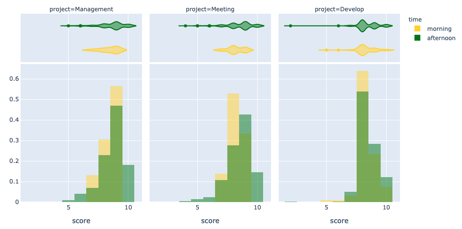
위의 상관관계들을 보았을 때, 아침 혹은 오후에 따라서 작업에 몰입하는 경향에 차이가 있음을 알 수가 있습니다. 집중도가 높으면서 기분이 좋은 경우를 몰입하는 상황(집중도 점수 + 행복도 점수)이라고 가정하고 작업들의 분포를 살펴보았습니다. 미팅/관리 쪽의 일들은 오전보다는 오후에 높은 점수 쪽으로 분포가 되어있고, 개발은 거의 비슷한 분포를 보이고 있네요.

이렇게 시간대에 따라서 영향을 받는 작업들이 있는 반면에, 아무런 상관관계가 없는 것도 있을 것입니다.
바로 ‘운동’ 입니다.

image.png

그림 7-1 평일 모든 시간대의 ‘운동’ 대한 상관계수

운동의 특성상, 언제 시작을 하던 (0.08), 혹은 얼마나 하던 (-0.02), 집중해서 하게 되고, 하고 나면 상쾌하기 때문이 아닐까 싶습니다. 실제로 운동에 대한 작업들은 거의 대부분이 5점에 있습니다. 이 조커와 같은 운동에 대한 효과는 운동을 한 날과 하지 않은 날을 비교해보면 더 그 차이를 체감할 수 있습니다.

image.png

그림 7-2 운동 여부에 따른 바이올린 차트

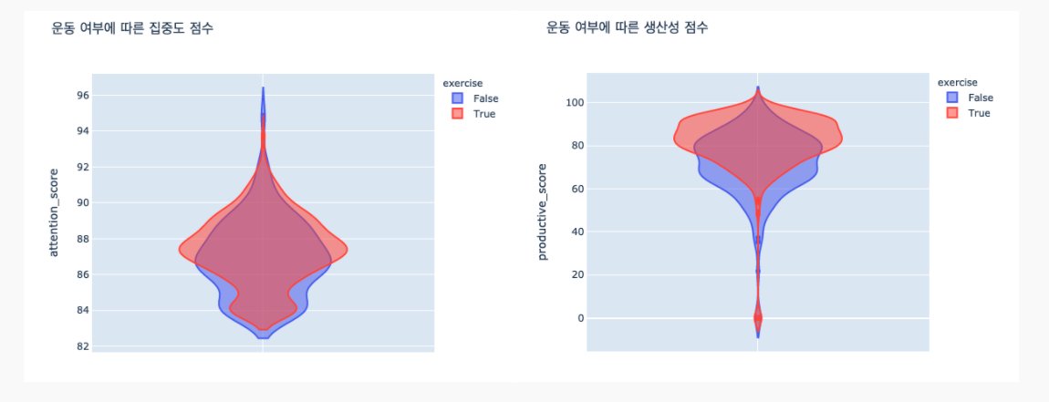
운동을 한 경우인, 빨간색 바이올린 도표가 조금 더 위로 위치해 있는 것을 볼 수 있습니다. 운동을 한 날이 하지 않는 날보다 조금 더 집중하는 편이고, 작업을 더 많이한다는 것을 말해주고 있습니다.

지금까지의 정보들을 종합해보면 다음과 같은 전략으로 하루의 작업들을 배치할 수 있을 것 입니다.

  • 오전에는 일찍 연구/개발을 시작해서 점심 먹기 전까지 쭉 집중
  • 연구/개발 작업은 오래할 수 있는 시간을 충분히 확보하고 진행
  • 미팅/관리 작업들은 오전보다는 오후에 진행
  • 운동은 아무때나 일정에 맞춰서 하되, 꼭 해주기

자기계발에 해당하는 우선 순위 2 의 작업들

image.png

그림 8 – 우선순위 2에 해당하는 작업 카테고리의 월간 작업시간 막대 그래프

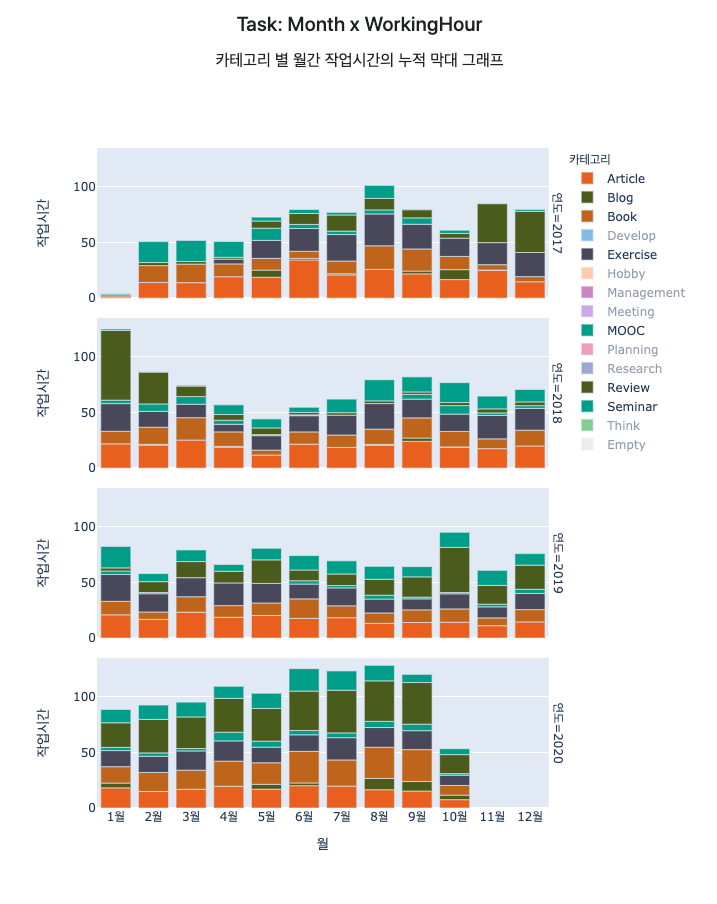
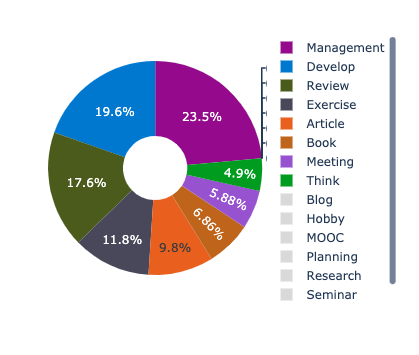
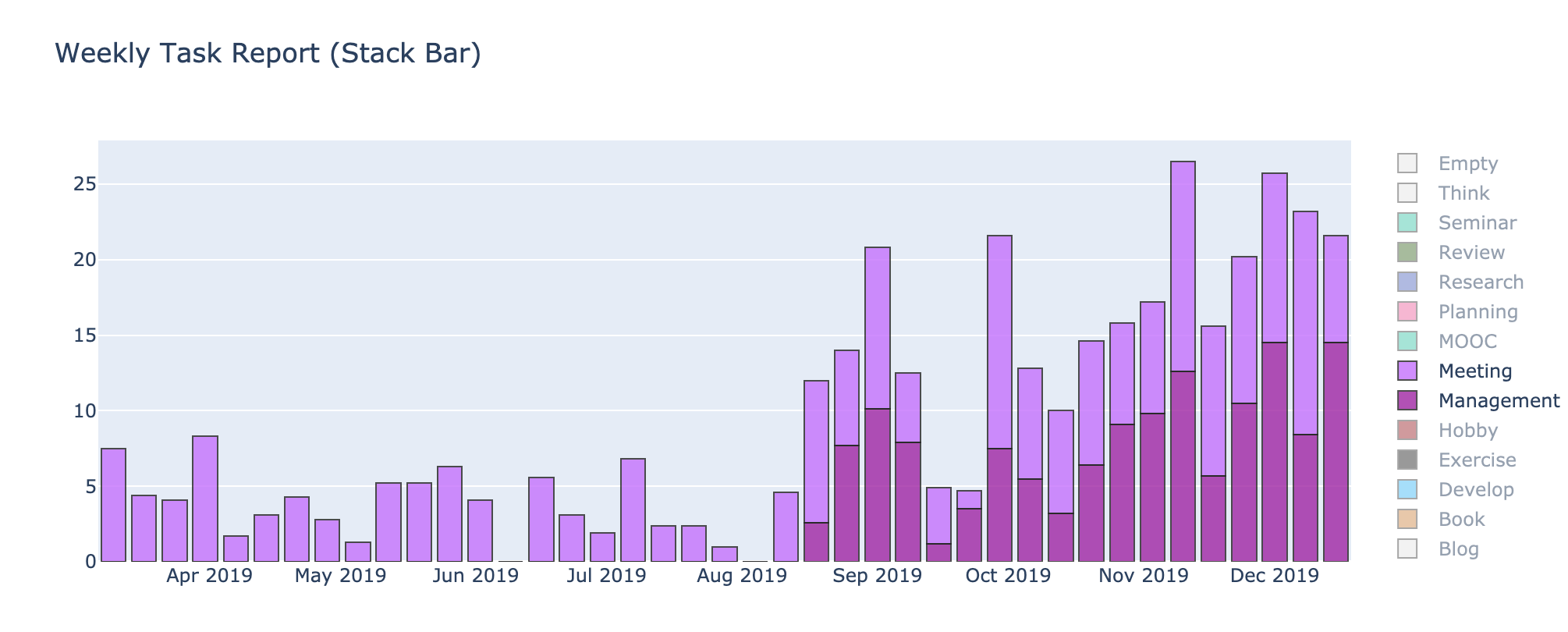
흔히 자기계발에 해당하는 시간들로 카테고리를 정리하였습니다. 여기에는 책을 읽고, 운동을 꾸준히 해주며, 각종 세미나와 강의를 듣고, 공부한 것을 정리하기도 하고, 일기를 쓰고, 명상을 하는 등의 다양한 활동들이 포함됩니다. 2018년 1월에 이상하게 데이터가 틔는 부분이 있지만, 전체적으로는 조금씩 시간을 늘려나가는 모습을 볼 수 있습니다. 명확한 목표 수치가 있는 것은 아니지만, 계속해서 공부를 하면서 꾸준히 월마다 80~100 시간은 쓰고자 하고 있습니다.

Metric은 고정이 아니라, 목표에 맞춰서 계속 변화합니다.

그 동안의 데이터를 분석해보니, 지금은 처음에 목표로 잡고 있던 Metric에는 근접한 생활을 하고 있다고 생각이 들었습니다. 이렇게 습관을 만드는 것이 어렵네요.

살면서 목표는 계속해서 변화하게 됩니다. 그에 따라서 Metric 또한 달라져야 할 것 입니다. 그리고 목표가 바뀌는 것 외에도 새로운 데이터를 수집할 수 있게 되거나, 기존의 데이터를 다른 방식으로 수집하게 된다면 이에 따른 목표 설정이 새로 필요할 것입니다. 현재 몇가지 변화를 주고 있는데, 가장 큰 변화는 아래 3가지 입니다.

image.png

출처: https://blog.fitbit.com/sleep-stages-explained/
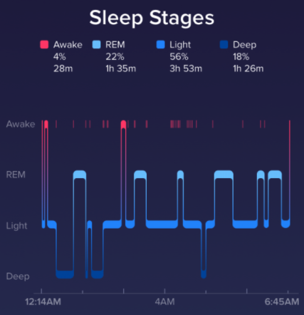
  1. 수면 : 현재는 Fitbit Versa 를 통해서 조금 더 정확한 수면에 대한 정보를 얻고 있습니다. 개인적으로 잠에 대한 관심도 많고, 가끔 밤에 잠이 안 와서 밤잠을 설친 날에는 그날 하루가 피곤해지는 것을 경험하다보니.. 자연스럽게 수면에 대해서 점수도 더 올리고 엄격한 기준을 적용해보려고 하고 있습니다.
    위의 그래프에서 보는 것처럼, 잠은 REB, Light, Deep 의 단계를 순환하고 그것을 잡아주고 있기 때문에 더 정확한 진단이 가능할 것입니다. 그 동안은 단순히 잠을 자기 시작한 시간, 일어난 시간을 기준으로 했기 때문에 수면시간과의 상관관계도 더 정확히 알아볼 수 있을 것입니다.
  2. 블로그 작성 : 많은 개발자분들에게 블로그는 꾸준히 해보려고 하지만 정말 잘 안되는 것 중의 하나일 것이라고 생각합니다. 저에게는 특히 그랬네요. 최근에는 글로 자신의 생각을 정리해보는 것이 정말 중요하고, 저만의 컨텐츠를 만들어보고 싶다는 생각으로 노력을 해보고 있습니다.
    블로그는 특별히 습관으로 만들기 위해 신경 쓰는 부분이라 habit 에 포함시켜서 진행 시, 5점을 주도록 설정하였네요. (다른 습관들은 자리를 잡아서 점수를 줄였습니다. 5→3점)
  3. 작업의 질 : 지금까지 집중했던 것은 ‘일단 하자’ 였습니다. 어느정도는 습관으로 자리를 잡은 지금은 ‘더 잘하자’ 에 포커스를 맞춰보고자 합니다. 작업의 질에 집중하는 이유는 의 한 구절을 인용해 보고자 합니다. 이제야 A작업을 어느정도는 해냈고, B 작업을 할 수 있는 단계가 되었다고 생각하기 때문입니다.함께>

    더글러스는 작업을 세 가지 수준으로 구분합니다. A, B, C 작업입니다.
    A 작업은 원래 그 조직이 하기로 되어 있는 일을 하는 걸 말합니다.
    B 작업은 A 작업을 개선하는 걸 말합니다. 제품을 만드는 사이클에서 시간과 품질을 개선하는 것이죠
    C 작업은 B 작업을 개선하는 것 입니다. 개선 사이클 자체의 시간과 품질을 개선하는 것입니다. … 한마디로 개선하는 능력을 개선하는 걸 말합니다.
    더글러스는 “우리가 더 잘하는 것을 더 잘하게 될수록 우리는 더 잘하는 걸 더 잘 그리고 더 빨리 하게 될 것이다” – 복리의 비밀, 34 페이지 중

끝으로

이번 포스트에서는 ‘생산적인 하루’ 를 정량적으로 수치화해보고, 직접 정의를 해본 Metric으로 점수를 산정해보았습니다. 그 동안의 데이터를 살펴보면서, 예전에는 더 열심해 했었는데.. 라는 생각도 하고 조금 더 자세히 데이터들을 분석해보면 하루를 조금 더 효율적으로 보낼 수 있는 방향도 알아보았습니다. 무엇보다도 저 자신을 더 이해할 수 있었습니다. 또한 2020년이 되어서야 데이터를 모으는 것에 그치지 않고, 한 걸음 더 나아갈 수 있었습니다. 가장 중요한 것은 액션 즉, 행동이기에, 이렇게 자신에 대한 데이터들을 통해 현실을 제대로 인지하고 그에 따라서 조금 더 나은 방향으로 행동에 변화를 이끌어 낼 수 있으면 좋겠습니다.
여러분의 하루는 어떤 식으로 수치화를 할 수 있을까요? 또 데이터에서 어떤 것들은 얻고 있으신가요?

Categories
Offsites

Quantified Self Part 5 – 데이터 시각화와 대쉬보드 with KPI

Kino 프로젝트는 QS를 통해서 자신에 대해서 알고, 불필요한 일들을 자동화시키고 삶의 질을 증진시키기 위한 프로젝트 입니다. 이번 편에서는 그 동안 모아온 데이터에 대한 시각화와 대쉬보드에 대해서 다뤄보고자 합니다.

images

출처 : http://quantifiedself.com/

지금까지의 시리즈

Github: https://github.com/DongjunLee/quantified-self

데이터 시각화와 대쉬보드가 필요한 이유

어떠한 문제를 해결하고 싶다면, 어떻게 풀어나갈 것인지 생각하는 것보다 중요한 것은 문제 자체에 조금 더 파고 들어가 그 문제를 제대로 이해하는 것입니다. 저는 지금까지 QS 프로젝트를 진행하면서 여러가지 데이터들을 쌓아왔습니다. 데이터 종류에는 각종 작업들에 대한 데이터와, 행복도, 잠에 대한 것들을 포함되어 있습니다. 기본적으로 시계열 데이터의 형식으로 되어있으나, 다양한 범주로 구성되어 있을 것 입니다. 이러한 데이터에서 실제 문제를 발견하는 가장 좋은 방법이 무엇일까요?
바로 ‘시각화(Visualization)’ 입니다.

어떻게 시각화를 하였는지 바로 넘어가기 전에 ‘시각화’ 에 대해서 조금 더 이야기 해보는 것이 글을 이해하는데 있어 도움이 될 것 같습니다. ≪데이터 시각화 교과서≫ 라는 책을 지은 클라우스 윌케는 데이터 시각화에 대해 다음과 같이 이야기하고 있습니다.

데이터 시각화는 다양한 의미가 담긴 숫자들을 점으로, 선으로, 면으로 그려내는 작업입니다. 수학적 언어를 시각적 언어로 ‘번역’하는 작업이죠.

이렇게 숫자를 ‘보는’ 언어로 바꿔서 우리에게 보여주는 이유는 데이터가 가지고 있는 무언가를 알아내기 위함입니다. 윌케는 시각화에 목적에 대해서는 이렇게 이야기합니다.

데이터를 시각화하는 목적은 주로 소통이다. 우리에게는 데이터셋에서 얻은 통찰(insight)이 있고, 잠재 독자가 존재하며, 우리가 얻은 통찰을 독자에게 전달하고자 한다. 통찰한 결과를 성공적으로 알리려면 독자에게 의미 있고 흥미로운 이야기를 들려줘야 한다.

이번 시각화에서의 독자는 저 자신이며, 하루하루 지내면서 지나쳤던 삶의 패턴들을 발견하고 다양한 통찰을 스스로에게 전달하는 것이 목적이 될 것입니다.

그리고 몇가지 차트들을 엮어서, 화면을 구성하는 것을 보통 대쉬보드(Dashboard)라고 합니다. 위키백과에서는 대쉬보드를 다음과 같이 설명합니다.

대시 보드는 특정 목표 또는 비즈니스 프로세스와 관련된 주요 성과 지표를 한 눈에 볼 수있는 그래픽 사용자 인터페이스 유형입니다.

이 QS 프로젝트의 대쉬보드 역시, 저 스스로 목표로 하는 주요 성과 지표를 한 눈에 볼 수 있어야 할 것입니다.

Python 시각화 라이브러리, Ploty

Quantified%20Self%20Part%205%20-%20Dashboard%2079c29c2ae22e47fdb65d96843a8a2566/Untitled.png

시각화 및 대쉬보드에 사용된 라이브러리는 ploty 라는 라이브러리 입니다. 차트를 그리는데 있어서는 matplotlib 을 기본으로 다양하게 사용되기는 하지만, plotly를 선택한 이유는 다음과 같습니다.

  • Plotly는 대쉬보드 용 프레임워크인 Dash 와 호환되어 지원합니다.
  • 간단하게 Interactive 차트를 구현할 수 있습니다.

(Plotly에 적혀있는 소개 한 문장: The interactive graphing library for Python (includes Plotly Express)

최근에 업데이트 된 것과 더불어서 간단히 소개를 더 드리자면, 최근에는 Plotly Express 가 업데이트 되면서 다양한 차트들을 더 간단하게 그릴 수 있게 되었습니다.

import plotly.express as px

df = px.data.gapminder()
fig = px.scatter(
    df.query("year==2007"),
    x="gdpPercap",
    y="lifeExp",
    size="pop",
    color="continent",
    hover_name="country",
    log_x=True,
    size_max=60
)
fig.show()

Quantified%20Self%20Part%205%20-%20Dashboard%2079c29c2ae22e47fdb65d96843a8a2566/Untitled%201.png

이미치 출처: https://plotly.com/python/plotly-express/ (링크에서는 Interactive Chart로 경험하실 수 있습니다.)

이제 도구가 정해졌으니, QS 데이터를 시각화에 대해서 설명드리고자 합니다.

QS를 위한 데이터 시각화

먼저 수집하고 있는 데이터에 대해서 알고 있어야, 무엇을 어떻게 시각화할 것인지 결정할 수 있을 것 입니다. 아래 데이터는 하루를 기준으로 수집되고 있는 데이터의 예시입니다.

  • record: 2020-08-07.json
{
    "activity": {
        "task": [
            {
                "toggl_id": 123,
                "start_time": "2020-08-07T00:27:45+09:00",
                "end_time": "2020-08-07T00:54:23+09:00",
                "project": "Review",
                "description": "...",
                "color": "#566614"
            },
            {
                "toggl_id": 124,
                "start_time": "2020-08-07T00:55:22+09:00",
                "end_time": "2020-08-07T01:05:54+09:00",
                "project": "Article",
                "description": "...",
                "color": "#e36a00"
            },
            ...
        ],
        "happy": [
            {
                "time": "2020-08-07T14:40:17+09:00",
                "score": 4
            },
            {
                "time": "2020-08-07T21:20:26+09:00",
                "score": 5
            }
        ],
        "sleep": [
            {
                "is_main": true,
                "start_time": "2020-08-07T01:52:00.000",
                "end_time": "2020-08-07T09:25:00.000"
            }
        ],
    },
    "summary": {
        "habit": {
		        "exercise": true,
		        "bat": true,
		        "diary": true,        
        },
        "productive_details": {
            "rescue_time": 91.25,
            "toggl": 100.0,
            "github": 40.0,
            "todoist": 88.0
        },
        "attention": 87.6,
        "happy": 96.0,
        "productive": 87.12,
        "sleep": 100.0,
        "repeat_task": 85.0,
        "total": 96.76
    }
}
  • activity: 활동에 대한 로그들을 담고 있습니다. 활동로그의 대표는 task , happy 그리고 sleep 입니다. 그 외에는 in_home, out_company 등.. 출퇴근 시간을 자동으로 추가한 로그 또한 포함되어 있습니다.
  • summary: 각 점수 기준에 맞춰서 계산된 점수들을 기본으로 가지고 있습니다. (계산하는 점수에 대해서는 다음 포스트에서 설명드릴 수 있도록 하려고 합니다.) 추가로 제가 중요하게 생각하는 habit 즉, 습관에 대한 기록 또한 true 혹은 false 로서 저장이 됩니다.

Daily Schedule

Quantified%20Self%20Part%205%20-%20Dashboard%2079c29c2ae22e47fdb65d96843a8a2566/Untitled%202.png

이 차트는 Gantt Chart 를 응용한 것으로서, 각 시간에 대한 작업들을 보여줍니다. 여기서 Y축은 집중도 로서 1~5점의 점수를 가지고 있습니다. 여기에 행복도 점수(초록색 동그라미)까지 더 해줌으로써, 어떤 작업들을 얼마나 집중하며 진행하였는지 그리고 각 시간 때의 기분에 대해서도 알 수가 있습니다. 하루를 대략적으로 돌아보기에 효과적인 차트입니다.
(원래 상세내역은 작업에 대해서 적혀 있지만, 위 차트에서는 ‘…’ 으로 표현하고 있습니다.)

Quantified%20Self%20Part%205%20-%20Dashboard%2079c29c2ae22e47fdb65d96843a8a2566/Untitled%203.png

Pie Chart 는 비율을 보는 용도로 사용이 됩니다. 위의 Daily Schedule과 함께 하루에 어떤 작업을 위주로 하였는지 알 수가 있죠. 여기서 비율은 작업의 시간을 기준으로 합니다.

Daily Habit

Quantified%20Self%20Part%205%20-%20Dashboard%2079c29c2ae22e47fdb65d96843a8a2566/Untitled%204.png

습관은 Heatmap 을 사용합니다. 보통 히트맵은 색상으로 각 데이터의 수를 표현할 때, 많이 사용합니다. 습관을 나타냄에 있어서 히트맵을 사용한 이유는 사실 단순합니다. Github의 개인 Contribution Chart와 같은 컨셉으로 만들고 싶었기 때문입니다.
이와 같이 만든 이유는 ‘일일커밋’ 때문입니다. 하루하루 꾸준히 커밋을 하는 것 역시 습관이라고 말할 수 있습니다. 위의 네모칸을 초록색으로 꽉 채우는 것이 습관을 잘 지켜 나가고 있다는 것을 보여줄 것입니다. 위 이미지의 기간 때에는 일기는 꾸준히 쓰지만, 운동은 중간중간 쉴때가 있고, BAT(공부한 것 정리)는 목표만 있지 실행되지 않던 때 이네요.

  • 참고) Github Contribution Chart

Quantified%20Self%20Part%205%20-%20Dashboard%2079c29c2ae22e47fdb65d96843a8a2566/Untitled%205.png

이미지 출처: https://github.com/jbranchaud/commitart

Daily Summary

Quantified%20Self%20Part%205%20-%20Dashboard%2079c29c2ae22e47fdb65d96843a8a2566/Untitled%206.png

각 날짜 별로 summary 에 포함되어 있는 점수들이 Line Chart 로 표현이 됩니다. 이 값들을 통해서 어떤 것이 잘 지켜지고 있고, 아닌지 점수로서 확인을 할 수 있습니다. 간단하게 보았을 때, repeat_task 의 점수가 보통 가장 낮은 점수를 받고 있음을 알 수 있습니다. 보통 이 차트를 부면서 ‘가장 부족한 부분을 하나씩 끌어올려야겠다.’ 고 자신을 푸쉬하게 됩니다.

Task Report (Daily/Weekly)

하루 혹은 일주일을 기준으로 진행한 Task들을 Stacked Bar Chart 로 시각화합니다.

Quantified%20Self%20Part%205%20-%20Dashboard%2079c29c2ae22e47fdb65d96843a8a2566/Untitled%207.png

이러한 누적막대 그래프는 기준에 따라서 (하루 혹은 월요일~일요일까지의 일주일)의 시간 총량을 알 수 있으며, 각 카테고리 별 시간의 합 그리고 각각의 날들을 비교하기에 좋은 시각화 방식입니다. 위의 차트를 보았을 때, 미팅을 몰아서 하려는 성향과 개발에 대한 시간이 꾸준하게 포함되는 것을 확인할 수 있습니다.

주요 성과지표 관리 (KPI)

위의 각각의 차트들은 실제로 제가 어떻게 생활을 해왔는지에 대해서 시각적으로 말을 해주게 됩니다. 하지만 이 차트들은 바로 보자마자 1) 하루를 생산적으로 보냈는지, 2) 습관으로 만드려고 하는 목표들이 제대로 지켜지고 있는지 명확하게 말해주지 않습니다. 예를 들어, ‘일주일에 5시간 이상은 책을 읽겠다’ 라는 목표를 확인하기 위해서는 주간 Task Report 에서 Book 카테고리의 시간을 직접 확인해봐야 합니다. 그래서 위의 시각화와는 별개로 주요 성과지표를 명확하게 확인할 수 있는 대쉬보드를 따로 개발하였습니다.

먼저 성과의 기준을 가지고 있는 kpi.json 파일이 있습니다.

{
  "daily": {
    "task_hour": [5, 8],
    "exercise": ["X", "O"],
    ...
  },
  "weekly": {
    "book": [2.5, 5],
    ...
  }
}

기준은 단순합니다. 각각의 항목에 대해서 왼쪽은 숫자의 경우 최소값, 오른쪽은 목표로 하는 수치입니다. 위의 값을 예시로 든다면, daily.task_hour 의 경우는 ‘최소 5시간 에서 최대 8시간 정도를 작업에 사용하라’ 는 지표를 의미하게 됩니다. 숫자가 아닌 daily.exercise 의 경우에는 운동을 안 했으면 X, 했으면 O로 인식이 될 것입니다. 이렇게 스스로 정한 KPI 에 맞춰서 대쉬보드가 제대로 하고 있는지 보여줍니다.

Quantified%20Self%20Part%205%20-%20Dashboard%2079c29c2ae22e47fdb65d96843a8a2566/Untitled%208.png

위의 보는 것처럼, Task Hour는 8시간을 넘어서 KPI를 달성했으므로 초록색으로, Diary의 경우는 아직 진행하지 않았기 때문에 빨간색으로 경고를 주고 있습니다. 위 대쉬보드는 Daily(하루 기준) 예시로서 Weekly(일주일 기준) 에서는 각 Task의 종류 별로 시간을 다루고 습니다. 예를 들어, KPI 첫 문단에서 이야기한 ‘일주일에 책 5시간은 보기’ 이러한 목표를 Weekly 대쉬보드로 확인할 수 있는 것입니다.

끝으로

그 동안 QS 프로젝트를 진행하면서, 데이터를 계속해서 모으고 있었습니다. 하지만 이 데이터들을 2020-08-07.json 과 같이 단순 텍스트 저장되어 있기 때문에 문제점을 정확하게 파악하고 있지 못했습니다. 대쉬보드를 만들면서 다양한 시각화 차트들을 그려보고 나니 실체가 적나라하게 보이는 느낌이였습니다. 이때 생산성 높은 생활패턴을 만드는 것과는 거리가 멀게 행동하고 있음을 알 수 있었습니다. 이것이 저에게는 데이터의 패턴을 변화시키는 자극제가 되어주었습니다. (물론, 계속해서 대쉬보드를 보다보면, 이것 또한 자극이 없어질 수도 있습니다..!) 글의 시작에서 이야기한 것처럼, 문제를 해결하기 위해서는 제대로 문제를 이해하는 것이 중요함을 다시 한 번 강조하고 싶습니다.
다음 포스트에서는 이 프로젝트의 1차 정리로서, 목표로 해왔던 ‘좋은 습관 만들기’ 에 대해서 지금까지의 데이터를 기반으로 정리해보려고 합니다.

Categories
Offsites

Product Manager를 위한 교과서, 인스파이어드

제품에 관한 책을 추천받을 때 항상 가장 먼저 추천하는 책이 있습니다. ‘인스파이어드’라는 책으로 마티 케이건의 저서입니다.

마티 케이건은 기술 제품 관리(Technology Product Management) 분야의 선구적인 사상가이자 실리콘밸리 제품 그룹(SVPG)의 창업자입니다. 또한 그는 HP, 넷스케이프, 이베이 등 세계 최고의 기업에서 제품을 정의하고 구현하는 책임자급 임원으로 근무한 경력이 있다고 합니다.

이 책에서는 Product Manager(제품 관리자)과 Product Team(제품팀)에 대해서 주로 이야기를 하고 있습니다. 개인적으로는 옮긴이의 말에 있는 문구가 이 책을 아주 잘 설명하고 있다고 생각합니다.

몇 년이 지난 지금까지도 ≪인스파이어드≫는 참고서처럼 수시로 꺼내 보게 되는, 제품 관리자로서 배우고 성장하는 데 도움을 준 가장 기본적인 안내서입니다. – 옮긴이 머리말 중에서

images

이미치출처: https://www.aladin.co.kr/shop/wproduct.aspx?ItemId=176659275

Product Manager는 CEO의 역할과 가장 비슷하다.

그렇다면 마티 케이건이 말하는 제품관리자는 어떤 사람인지 한번 들어보시죠.

이 책을 관통하는, 내가 확신하고 있는 중심적인 개념이 있다. 바로 모든 훌륭한 제품 이면에는 지칠 줄 모르고, 무대 뒤에서 최선을 다하는 누군가가 있다는 것이다. 그 사람은 제품팀을 이끌며, 비즈니스 목표에 맞는 방향으로 기술과 디자인을 통해 고객의 실제 문제를 해결한다. 이런 사람들을 우리는 제품 관리자(product manager)라고 부른다.
… (중략)
나는 주어진 업무를 충실하게 수행하면서 주 60시간보다 적게 일하는 제품 관리자를 많이 보지는 못했다.

뛰어난 제품 관리자는 네 가지 중요한 책임을 다 한다.

  1. 고객에 대한 깊은 이해: 제품 관리자는 실제 제품에 대해 모두가 인정하는 전문가가 되어야 한다.
  2. 데이터에 대한 깊은 이해: 오늘 날 제품 관리자는 데이터와 분석 정보에 익숙해야 한다. … 데이터를 분석하고 고객을 이해하는 일은 다른 사람에게 맡기면 안 된다.
  3. 비즈니스에 대한 깊은 이해: 성공적인 제품은 고객에게 사랑받는 것은 물론이고, 사업적인 성과도 함께 창출한다.
  4. 시장과 산업에 대한 깊은 이해: 당신이 경쟁하고 있는 시장과 산업에 대한 깊이 있는 지식이다.

피터 드러커의 ≪매니지먼트≫에서 매니저를 ‘조직의 성과에 책임을 지는 자’ 라고 정의한 것처럼, 케이건은 Product Manager를 ‘제품을 완성하는 것에 그치는 것이 아니라 비즈니스 성과를 책임지는 자’라고 말하고 있습니다. CEO의 역할과 가장 비슷하다고 말하는 이유이기도 합니다.
또한 마티 케이건은 Product Manager는 누구보다 똑똑하고 창의적이며, 집요한 사람이어야 하기에 이는 자 이여야 한다고 말하고 있습니다. 비즈니스에 대한 성과를 만들 수 있다는 것은 곧 제품 백로그에 있는 일이 만들만한 가치가 있는지 확실할 수 있다는 뜻이기도 하기 때문입니다.

진정으로 제품팀이 전부다.

다음으로 저자가 특히 강조하는 ‘제품팀’ 에 대한 설명입니다. 제품팀에 대해서는 책의 전반에 걸쳐서 다뤄지고 있고, 이는 제품팀이 훌륭한 제품을 만드는 데 있어 얼마나 필수적인 요소인지를 말하고 있다고 생각합니다.

제품팀은 아마도 이 책 전체에서 가장 중요한 개념일 것이다. 진정으로 제품팀이 전부다.

존 도어 (John Doerr)의 말이 제품팀의 목표를 가장 잘 표현한다. “우리가 원하는 것은 용병팀이 아닌 미션팀(team of missionary)이다.” 용병팀은 지시한 것만을 만든다. 미션팀은 진심으로 비전을 믿고 그들의 고객 문제 해결을 위해 최선을 다한다.

위의 존 도어의 말은 제품팀을 정의하는 데 있어서 가장 중요한 문장일 것입니다. 제품팀은 미션팀 이여야 한다는 것. 그리고 제품을 만들어본 사람들이라면 용병팀과 미션팀이 보여주는 모든 차이에 대해서 이해할 수 있을 것입니다.

기억하라. 제품팀의 가장 중요한 속성은 용병이 아닌 미션팀을 원한다는 것이다. 이것은 주인 의식과 자율성의 개념과 직접 연관되어 있다. 팀이 충분한 권한을 가지고 있고, 제품에서 중요한 부분을 책임지고 있다는 것을 느낄 수 있어야 한다. … 우리는 최대한의 자율성을 위해 늘 최선을 다해야 한다.

스타트업은 이러한 제품팀의 관점으로 바라본다면, 다음과 같을 것입니다.

“오직 우리만이 저 문제를 제대로 풀 수 있고, 이 문제를 풀어서 고객에게 가치를 준다.” (How to Start a Startup – Stanford에서 말하는 스타트업의 창업자에 대한 강의에서 인용하였습니다)

저는 제품팀이 만들어지는 것은, 창업한 후에 약 10명 규모가 되기까지 초기 직원들을 고용하는 과정에 가깝다고 생각을 합니다. 초기에 꾸려지는 제품팀의 팀원들은 만들고자 하는 제품에 대한 비전을 믿으며, 개개인이 가지고 있는 능력 또한 출중한 사람일 것이기 때문입니다.
여기서 특히 중요한 것은 제품의 미션을 믿는 것입니다. 능력에 대해서는 개개인의 노력에 해당하는 일이지만, 해결하고자 하는 문제와 제품에 대한 비전을 팀원들에게 관철되도록 하는 것은 제품 관리자가 꼭 해야 하는 일이기 때문입니다. (이것이 가장 어려운 일이 아닐까 싶기도 합니다) 또한 다시 한번 말하지만, 용병팀과 미션팀은 일을 진행하는 방식과 퍼포먼스 그리고 일을 진행하면서 배우는 학습까지 모든 것이 다르기 때문이기도 합니다.

제품에 대한 기본적인 안내서

처음 이 책을 소개할 때, 이 책을 ‘제품 관리자로서 배우고 성장하는 데 도움을 준 가장 기본적인 안내서’ 라고 이야기했었습니다. 바로 ‘각각의 역할’, ‘제품’ 그리고 ‘프로세스’ 에 대해서도 다루고 있기 때문입니다.

제품 관리자, 디자이너와 엔지니어, 제품 로드맵과 전략, 원칙 그리고 OKR 등 프로세스에서는 제품 발견부터 프로토타이핑과 발견한 제품에 대한 테스트, 이후의 프로세스 확장까지 다양한 주제에 관해서 이야기를 합니다. 하나하나 깊이 들어가는 것보다는 하나의 주제에 대해서 핵심이 되는 부분을 이야기합니다.

또한, 단순하게 제품을 만들어 가는 과정만을 이야기하는 것이 아닌, 각 회사 크기에 대한 접근법과 특징들, 제품 로드맵, 출시되기까지의 전체 프로세스, 이해 관계자의 관리 역시 중요함을 이야기하고 있습니다. 어느 규모에서든 제품을 만들어본 경험이 있으시다면 자연스럽게 공감할 수 있는 내용 또한 담겨 있습니다.

마지막으로 무엇보다 어려운 일은 훌륭한 제품을 계속해서 만들 수 있도록 환경을 만드는 일일 것입니다. 저자는 마지막 파트로서 ‘문화’를 이야기합니다.

이 책에서 진정으로 말하고자 하는 것이 바로 제품 문화라는 것을 당신이 느꼈을 것으로 생각한다. … 나는 제품 문화를 두 가지 관점으로 바라본다. 첫 번째 관점은 회사가 고객을 위해 가치 있는 솔루션을 만들어 내기 위해 끊임없는 혁신을 할 수 있느냐는 것이다. 이것이 바로 제품 발견이다. 두 번째 관점은 실행이다. 아무리 훌륭한 아이디어라도 만들 수 없고 고객에게 전달할 수 없는 버전이라면 아무 소용이 없다. 이것이 바로 제품 실행이다.

끝으로

저 역시 이 책을 프로젝트 중간중간 참고하기도 하면서 제품이 제대로 나아갈 수 있도록, 비행기의 항로를 조절하듯이 계속해서 방향을 잡기 위해 노력을 하곤 합니다. 프로젝트에서 실제로 무슨 역할을 맡고 있던, 제품에 대한 제대로 된 시각과 접근법을 알고 있다면, 일하면서도 더욱더 많은 것을 배울 수 있으며 그 자체로 훌륭한 제품을 만드는 데 한 걸음 더 다가간 것으로 생각합니다.

저자가 강조한 것처럼 저 역시 제품팀이 전부라고 생각을 합니다. 자신이 만드는 제품에 대한 애정을 가지며, 실제로 사용자에게 가치를 줄 수 있는 제품을 내보이는 것. 단순한 문장이지만… 정말로 어려운 일이고, 제대로 하고 싶은 일 이기도 합니다.

이 책에 있는 벤 호로위츠의 ‘(좋은 제품 관리자/나쁜 제품 관리자)’ 의 일부로 글을 마무리하고자 합니다.

  • 좋은 팀은 강렬한 제품 비전이 있고, 그들은 마치 선교사와 같은 열정을 추구한다.
    나쁜 팀은 용병들이다.
  • 좋은 팀은 어떤 아이디어가 진정으로 만들 만한 가치가 있는지를 결정하기 위해 빠르게 제품 아이디어들을 시도해 볼 수 있는 많은 기법에 능숙하다.
    나쁜 팀은 우선순위 로드맵을 만들기 위해 미팅을 진행한다.
  • 좋은 팀은 최종 사용자 및 고객과 매주 직접 만난다. 그리고 최신 아이디어에 대한 고객들의 반응을 확인한다.
    나쁜 팀은 그들 자신이 고객이라고 생각한다.
  • 좋은 팀은 속도의 중요성과 빠른 이터레이션이 혁신의 핵심임을 이해하고 있다. 그리고 이러한 속도는 일의 양이 아닌 올바른 기법을 사용하는 것에서부터 시작되는 것임을 안다.
    나쁜 팀은 그들의 동료가 충분히 최선을 다하지 않는 것이 속도가 느린 원인이라고 불평한다.

부록

  • 2019년 11월 5일에 ‘Product is Hard’ 라는 주제로 마티 게이건이 강연을 하고, 정리가 잘 된 좋은 글이 있어서 추가합니다. (https://medium.com/@kevinsohn/product-is-hard-marty-cagan-2df47835aa1d)

  • Wanted Con : Product & Strategy 에서 라인 서비스 플래너 옥지혜님이 ‘지금 프로덕트 매니저는 무슨 일을 하고 있을까?’ 라는 주제로 이야기한 세션에서 공감가는 내용이 있어서 덧붙입니다.

    제품은 PM과 제품팀이 버텨서 성공할 수 있는 것이 아닌가… 제품의 한계는 제품팀의 한계와 같다.

Categories
Offsites

아주 늦은 2019년 회고

개인적으로 간단하게 작년 연말에 회고를 하였지만, 블로그를 제대로 시작할 겸..!
2019 회고글을 작성해보고자 한다. 생각보다 시간이 지났기 때문에 당시 회고하면서 바라보는 관점과 지금의 관점은 약간의 차이가 있을 수는 있을 것 같다.

회사

그 어느 때보다도 회사의 일에 집중을 했던 한해라고 생각을 한다.
매일 매일 되도록이면 일기를 쓰려고 하는데, 지금 돌아가서 그때의 일기들을 들여다보면 회사에서 느꼈던 감정들이 대부분인 정도이다. 그래서 2019년 회고는 회사 관련한 글이 많지 않을까 싶다.

LaRva 프로젝트와 PM

18년도 10월에 BERT라는 논문이 공개되고, NLP 분야에서는 바야흐로 BERT의 시대가 되었었다. 논문의 abstract에도 다음의 문구가 포함되어 있을 정도이다.

It obtains new state-of-the-art results on eleven natural language processing tasks

“물 들어올 때, 노 저어라” 라는 말처럼, 이 BERT 모델의 급 물살을 탈 수 있었던 프로젝트가 LaRva 프로젝트이다. (이 자리를 빌려, 프로젝트를 셋팅하고 PM을 맡겨주신 서민준님께 감사의 말씀을 드린다.)

최근에는 PM으로서, 제품에 대한 공부를 많이 하고 있다보니 지금의 시각으로 프로젝트를 돌아보려고 한다.
LaRva는 연구위주의 프로젝트이지만, 좋은 언어모델을 만드는 목적을 가진 하나의 제품으로서도 바라볼 수 있다고 생각이 든다.
다음은 ≪인스파이어드≫ 에서 제품 발견의 목적으로서, 아래 4가지 항목의 위험에 대비해야 함을 말하고 있다.

  • 고객이 과연 이 제품을 구매하거나 사용할 것인가? (가치 위험 Value Risk)
    ⇒ 다양한 NLP 서비스에 쉽게 적용할 수 있고, 성능을 올림으로서 서비스 품질에 기여할 수 있다는 것
  • 사용자가 이 제품의 사용 방법을 이해할 수 있는가? (사용성 위험 Usability Risk)
    ⇒ Github에 코드들이 계속 공개 되고 있었고 특히, huggingface에서 지금의 transformers 저장소를 만들어낸 것과 같이, 누구나 쉽게 쓸 수 있도록 정말 빠른 속도로 작업을 하고 있었다.
  • 우리가 만들 수 있는 것인가? (실현 가능성 위험 Feasibility Risk)
    ⇒ 가장 큰 제약은 GPU 일 것이다. 네이버이기 때문에 이런 제약은 해결이 될 수 있었다.
  • 우리 사업에 효과가 있는 솔루션인가? (사업 유효성 위험 Business Viability Risk)
    ⇒ 시간이 지나면서 이 BERT라는 모델의 중요성은 부각이 될 것이고, 이에 따라서 자연스럽게 풀릴 수 있는 문제라고 생각했다.

지금 와서 생각해보면.. 이렇게 잘 정의될 수 있는 프로젝트는 드물 것이라 생각을 한다.

위와 같이 위험한 부분이 없는 프로젝트로서 좋은 결과물들을 만들어 나아갈 수 있었고, KorQuAD v1 리더보드와 연말에는 Deview 2019 발표 그리고 사내 연구 아이템 2위로 선정이 되는 등 여러가지로 정말 얻은 것들이 많다고 생각한다.

2019%204d025a4489ba4870828420f0b38f75b6/Untitled.png

[KorQuAD v1 Leaderboard](https://korquad.github.io/category/1.0_KOR.html), Anonymous 때문에 힘들었던..

2019%204d025a4489ba4870828420f0b38f75b6/Untitled%201.png

출처 : https://www.pinterest.co.kr/pin/515662226060509153/

2019%204d025a4489ba4870828420f0b38f75b6/Untitled%202.png

출처 : https://m.mk.co.kr/news/english/view/2017/11/777734/

여담이지만, 프로젝트의 이름을 LaRva로 짓게 된 이유도 이야기해보려고 한다.
NLP에 계시는 분들은 ELMo, BERT, ERNIE 이런 식으로 네이밍을 하는 이유가 Sesame Street의 캐릭터들의 이름에서 가지고 왔다는 것을 알고 있을 것이다. 어쩌다보니 우리팀 역시 이러한 네이밍 트랜드를 따라서 국산 애니메이션 LaRva로 이름을 짓게 되었다. 지금도 참 입에 잘 붙고, 좋은 네이밍이였다고 생각을 한다.
(LaRva의 풀네임은 Language Representations by Clova 이다.)
그리고 실제로 이러한 네이밍이 가지는 영향에 대해서도 어느정도 실감할 수 있었다. KorQuAD와 Deview 등 모두 LaRva 라는 이름으로 리더보드에 등록하고, 발표를 진행하면서 하나의 팀으로서, LaRva는 어떠한 팀인지 브랜드를 구축했다고 본다.

그리고 또 한가지 나에게 이 프로젝트가 중요한 의미를 가지는 것은 PM 으로서의 커리어이다.
기존에는 팀에서 ML Engineer 로서 역할을 하고 있었지만, 새롭게 프로젝트가 정리되고 기존 팀이 나눠지면서 PM 제안을 받게 되었다.
시작은 나를 포함해서 총 4명으로 일을 진행했고, 매니징보다는 실무를 많이 보았었다. 소수이지만 모두 정말 잘하시는 분들이었기 때문에 위처럼 좋은 결과를 냈다고 생각한다. 그리고 당연하게도 좋은 결과를 내면서 PM이라는 Role에도 약간의 재미를 느꼈던 것 같다.
또한 이때는 이러한 PM이라는 역할이 더 나아가게 될지는 알지 못 했다…!

CLaF 오픈소스화

2019%204d025a4489ba4870828420f0b38f75b6/Untitled%203.png

CLaF(Clova Language Framework)는 Clova AI에 합류했을 때, 기존의 팀에서 진행했던 프로젝트이다. NLP 프레임워크로서 다양한 Task들을 셋팅하고 돌릴 수 있으며 각각의 Experiment 들을 Pipeline 화하여, 하나의 모듈 혹은 컴포넌트를 쉽게 만들 수 있도록 틀을 제공해주는 프레임워크로 설계하였다.

개인적으로 아쉬웠던 점은 Github을 살펴보면.. 다수의 ML/DL 관련한 프레임워크들이 오픈소스화 되어있었는데, 대부분이 미국회사였다. 특히 Google과 Facebook..! 이러한 여러 좋은 프로젝트들에 뒤지지 않는 좋은 퀄리티의 프레임워크를 만들어보고 싶었고, 특히 오픈소스를 만들어서 많은 NLP 종사자분들과 이야기하며 퀄리티도 올리고, 이력서의 하나의 아이템으로도 쓸 수 있도록 만들고 싶었다. 솔직하게, 기대보다는 관심을 받지 못 하였다. Github의 Star가 높다고 맹목적으로 좋다라고 말을 할 수는 없지만.. 관심과 영향도의 측면은 충분히 보여주는 지표라고 생각한다. 현재 기준으로.. Star 182개 이고 나 역시 유지보수에 시간을 사용하지 못하고 있으므로 확실히 정체가 되어있는 상황이라 볼 수 있다.

‘차별화’는 무엇이든 만들 때 적용되는 원리이다. 프레임워크를 만들때 역시 차별화를 확실하게 해야한다는 점을 뼈저리게 느꼈다. 혹은 선구자가 되거나. 사내의 팀용으로 처음 개발을 시작했기 때문에, 다양한 요구사항을 충족시키기 위해 점점 하나의 특징보다는 다양한 케이스를 커버할 수 있는 프레임워크가 되어갔고 이때, 가장 많이 참고했던 allennlp 와의 차별점을 가지지 못 했던 것 같다.

이렇게 비슷한 방향으로 프레임워크가 발전해 나아갔지만, AllenNLP의 경우 그때 당시에도 이미 유명한 프로젝트 였으며 이렇게 될 수 있었던 것은 2가지 요인이 있다고 본다. 첫 번째는 Zero to One 으로 당시에는 이 정도로 잘 만들어져있는 범용 NLP 프레임워크가 없었던 것. 다음으로는 allenai 에서 나오는 논문들이 이 프레임워크에서 릴리즈가 되기도 하면서 특히 수혜를 많이 보았다고 생각한다. ELMo가 대표적일 것이다. claf의 경우에는 후발 주자 이기도 하였고, 논문이 구현되는 등의 이런 수혜를 받을 수 없었기 때문에 어쩌면 당연한 결과일지도 모르겠다.

나에게는 다소 아쉬울 결과였다고 해도, 시작부터 끝까지 만들어나가면서 결국 오픈소스화까지 할 수 있었고 여기서 배운 것들은 매우 많다. 특히 설계부분에 대해서 신경을 썼고, 내부적으로 여러 PR들에 대해 이야기할 때도 설계자의 관점으로서 이야기를 할 수 있다는 것은 특별한 경험이기도 하였다. 앞으로 시간이 좀 날 수 있다면, 유지보수와 더불어서 확실한 색깔을 갖춰보고 싶다.

DUET PM 그리고 AiCall

2019%204d025a4489ba4870828420f0b38f75b6/Untitled%204.png

출처: [아웃백 미금점 AiCall 이벤트](https://clova.ai/m/ko/events/aicall/)

커리어측면으로 확실한 방향 전환이 일어난 사건이다. 사내에서 개발 중인 ‘전화를 대신 받아주는 AI 서비스’ 프로젝트인 DUET의 Project Manager를 9월 혹은 10월 쯤에 맡게 된 것이다. 기존 연구 중심의 LaRva 프로젝트와는 다르게 철저히 Product 중심의 프로젝트였기 때문에 내가 해야하는 역할 또한 기존과는 확실히 달랐다. 이때부터 실무를 볼 수 있는 시간이 급격하게 줄어드는 것이 느껴졌다…

해당 프로젝트는 이미 잘 셋팅이 되어있었기 때문에, 내가 주로 맡았던 일은 ‘제품 실행 관리자 (Delivery Manager)’ 에 가깝다. 어느 회사나 비슷할 것 같지만.. PM 이라는 역할은 필요한 일이면 무엇이든 하고 있는 사람이기에.. ≪인스파이어드≫에서 ‘제품 실행 관리자’ 의 역할을 다음과 같이 소개하고 있다.

제품 실행 관리자는 특별한 유형의 프로젝트 관리자로서 모든 장애물과 방해 요소를 없애는 임무를 가지고 있다. 때로는 다른 제품팀이 장애물이 되기도 하고, 어떤 경우는 제품 외부의 기능 조직이 되기도 한다. 하루 동안 그들은 여러 종류의 일을 해낸다. 마케팅 부서의 누군가를 찾아서 의사결정이나 승인을 요구하고, 다른 팀의 제품 실행 관리자와 협업하여 의존성이 있는 일에 대한 우선순위를 논의한다. … 제품 실행 관리자는 보통 팀의 스크럼 마스터 역할도 수행한다. … 채찍을 휘두르는 것이 아니라 일을 가로막는 방해 요소를 제거함으로써 이를 가능하게 한다.
━ 19. 제품 실행 관리자의 역할 중에서

모든 장애물과 방해 요소를 없애는 임무라.. 이미 들어가 있는 단어가 굉장히 위험하다고 생각이 든다. ‘모든’ 이라니… 그래도 이 한 문장은 PM의 특히나 중요한 임무이면서, 어려운 일을 이야기하고 있다. 위험 요소를 미리 파악하고 대처하며 제거한다는 것. 여기에는 굉장히 많은 일들이 포함될 수 있다. 성능이 안 나오는 컴포넌트의 성능을 올리는 일, 다른 부서와의 커뮤니케이션, 팀원 분들과의 면담과 계속해서 일하고 싶은 팀을 만드는 일 등 사실상 모든 일들이 포함될 수 있다.

그리고 조금 더 많은 인원의 PM으로 일을 하면서 느꼈던 점은 감정노동이 굉장히 많다는 것이다. PM의 기본적인 롤에서 한 가지는 사람을 적재적소에 배치해야 한다는 것이다. 이를 피터드러커의 ≪매니지먼트≫에서는 아래와 같이 이야기를 하고 있다.

가장 중요한 것은 실제로 행하는 일이다.

  • 일과 직장에 대해 성과와 책임을 부여한다.
  • 함께 일하는 사람들을 활용해야 할 대상으로 파악한다.
  • 강점이 성과에 결부되도록 사람을 배치한다.
    이에 따라 사람을 활용해야 할 대상으로 보고 적재적소에 배치할 수는 있을 것이다. 또한 조직의 목표가 온전히 업적으로 향하도록 만들 수도 있다. … 분명한 것은 신뢰와 성과가 눈에 보일 것이라는 점이다. 확신컨대 매니지먼트는 진정한 리더십으로 나아갈 수 있을 것이다.
    ━ 13. 사람이 최대의 자산이다 중에서

사람을 활용해야 할 대상으로 본다는 것은 얼핏보면 거부반응이 일어날 수도 있다. 하지만 이는 정확한 표현이라는 것들을 시간이 지나면서 실감하였다. 이렇게 일을 할 수 있다면, 자연스럽게 아래의 매니저가 해야하는 일 또한 달성이 가능하기 때문이다.

첫 번째 역할은 투입한 자원의 합계보다 큰 것을 만들어 내는 생산체를 조직하는 것이다.
두 번째 역할은 모든 결정과 행동에 있어 필요한 것과 미래에 필요하게 될 것을 조화시켜가는 것이다.
━ 20. 매니저의 일 중에서

그리고 많은 사람들이 함께 일을 하면 할 수록, 수 많은 문제가 생기기도 하고 그러한 문제를 팀원들을 모두 고려하면서 푸는 것이 기본이 된다. 이때에는 감정노동이 꼭 수반된다. 한창 힘들때, 감정노동 관련해서 공감과 위로를 받았던 부분이 ≪실리콘벨리의 팀장들≫ 에 있어 적어보고자 한다.

“제 일이 훌륭한 기업을 만드는 걸까요, 아니면 감정적인 보모 노릇을 하는 걸까요?”
“보모 노릇이 아닙니다. 그걸 관리라고 부릅니다. 바로 당신이 해야하는 일이죠!”

특히 위의 ≪실리콘 벨리의 팀장들≫ 이라는 책에서는 ‘완전한 솔직함’을 기준으로 신뢰관계를 구축하는 것의 중요성을 말하고 있는데, 이러한 신뢰관계가 구축할 수 있다면 팀내의 ‘심리적 안정감’ 역시 구축할 수 있을 것이라 생각을 한다.

여기서 ‘심리적 안정감’은 ≪두려움 없는 조직≫, ≪함께 자라기≫ 등의 책에서 많이 다뤄지는 개념이다. 김창준님이 저술하신 ≪함께 자라기≫ 에 있는 구절을 적어보자면 다음과 같다.

구글은 데이터 중심 회사답게 데이터 기반으로 뛰어난 관리자의 특징을 찾는 옥시전 프로젝트 이후에도 뛰어난 팀의 특징을 찾기 위해 2년간 노력했습니다. 이름하여 아리스토텔레스 프로젝트 입니다.

  1. 팀에 누가 있는지 (전문가, 내향/외향, 지능 등) 보다 팀원들이 서로 어떻게 상호작용하고 자신의 일을 어떻게 바라보는지가 훨씬 중요했다.
  2. 5가지 성공적 팀의 특징을 찾았는데, 그중 압도적으로 높은 예측력을 보인 변수는 팀의 심리적 안전감이었다.
  3. 팀 토론 등 특별히 고안된 활동을 통해 심리적 안전감을 개선할 수 있었다.
    ━ 구글이 밝힌 탁월한 팀의 비밀 중에서

이런 ‘심리적 안정감’ 개선하기 위한 특별한 활동들을 해보지는 못하였는데, 다음에는 기회가 되면 이러한 여러가지 활동을 해보는 것도 많은 것을 배울 수 있을 것이라 생각한다.

마지막으로 ≪매니지먼트≫ 에서 피터드러커가 말하는 매니저의 근본적인 자질에 대한 글로 PM 파트를 마무리하고자 한다.

먼저 사람을 관리하는 능력을 배워야만 한다. … 근본적인 자질이 필요하다. 바로 성실함이다.
조직원들에게 업무 처리를 일류로 해 낼 것을 요구하며 똑같이 엄격한 기준을 스스로에게도 적용한다. 기준을 높이 설정하고 그것을 지킬 것이라 기대한다. ‘무엇’이 옳은지만 생각할 뿐 ‘누가’ 옳은지는 생각하지 않는다. 성실함보다 지적 능력을 평가하는 일도 없다. … 매니저의 일은 체계적인 분석의 대상이다. 매니저가 할 수 있어야 하는 일은 그 대부분이 가르쳐 주지 않아도 배울 수 있는 것이다. 그러나 배울 수 없는 자질, 후천적으로 획득할 수 없는 자질, 처음부터 갖추고 있지 않으면 안 되는 자질이 한 가지 있다. 다시 말하지만 재능이 아니라 성실함이다.
━ 20. 메니저의 일 중에서

대외활동

Deview 2019 발표

2019%204d025a4489ba4870828420f0b38f75b6/Untitled%205.png

Deview 발표는 네이버로 이직을 했을 때부터 막연하게라도 생각해오던 목표 중 하나이다. 그 동안 Deview 에서 다양한 세션들을 들어오면서 한번 쯤은 발표자가 되는 것을 생각해보기도 하였고, 무엇보다 회사 내부에서 한 일을 외부에도 공유하고 알리고 싶었다. 개인은 물론이고, 팀의 기술력 또한 홍보할 수 있는 아주 좋은 기회이기에..!

엄~청 큰 언어 모델 공장 가동기! (LaRva: Language Representation by Clova)

위에서 다루었던 LaRva 프로젝트에 대한 발표였고, 굉장히 많은 분들께서 자리를 채워주셔서 BERT 라는 모델의 영향력이 어느정도 인지 실감할 수 있었다. 발표자료를 준비하면서.. 조금이라도 더 의미있는 시간으로 만들고 싶어서 욕심을 부리다보니.. 발표자료가 총 109장이 되었었다. 막상 발표 떄는 장수에 비해서 조금 빨리 마무리하기는 하였지만 그래도 잘 마무리 했다고 생각을 한다.

아쉬웠던 점은 결국, BERT 모델을 학습할 수 있는 것은 개인으로는 어려움이 있고 기업 특히, GPU 리소스가 풍족한 곳에서 가능한 일이기에 많은 분들에게는 실효성이 조금 적었을 수 있다. 이 분야에 종사하고 있는 분들에게는 도움이 될 수 있겠지만, NLP에 관심이 있는 정도라면.. 조금은 멀게 느껴졌을 수도 있다고 생각이 된다.

그래도 발표를 준비하면서 청중이 누구인지, 그리고 발표의 흐름이 매끄럽게 잘 이어지는지, 각 페이지의 설명이 충분한지, 시간 배분 등.. 이러한 다양한 포인트에 대해서 피드백도 받고 준비를 하면서 많이 배웠다고 생각한다. 20년에도 이렇게 인사이트를 공유할 수 있었으면..!

Quantified Self

주간 작업 리포트의 변화

약 3~4년 전에 사이드 프로젝트로 kino-bot 이라는 나 자신의 데이터를 수집하고, 반복되는 일들을 자동화 시켜주는 개인용 봇을 만들면서 계속해서 데이터를 수집해오고 있었다. 그 중 하나가 생산성을 측정하기 위해, 진행하는 일들에 대해서 시간을 기록하는 것이다.

Task의 카테고리들은 아래와 같다.

  • Seminar: 스터디, 강연 등
  • Review: 명상, 일기, TIL 정리, 회고, Deview 발표연습 등
  • Research: 논문을 포함한 연구관련 작업들
  • Develop: 개발관련 작업들
  • Planning: 계획
  • Meeting: 미팅..
  • Management: 프로젝트 관리에 해당하는 일들 (e.g. 칸반보드, 스크럼 운영, 문서 정리, 커뮤니케이션 등)
  • Exercise: 운동 (산책, 자전거 출퇴근, 요가, 근력 등)
  • Book: 종류에 상관없이 책을 읽는 경우
  • Article : 새로운 정보들을 확인하는 경우 (RSS 피드, 뉴스레터, 블로그, Reddit 등등)

2019%204d025a4489ba4870828420f0b38f75b6/Untitled%206.png

위 차트들은 주 단위의 Task 로서, 월요일부터 일요일까지의 Task들의 시간을 Stacked Bar Chart로 보여준다. 위 카테고리에 해당하는 시간들을 생산적인 일에 사용했다고 가정하고 시간을 기록해오고 있다.

이 차트를 보면, Role의 변화를 체감할 수 있다. 19년 초반에는 주로 Develop 에 대한 일들이 많았다면, 점점 시간이 지나면서.. 8월부터는 Management 라는 카테고리가 추가되기 시작했으며.. 시간이 갈수록 Meeting 과 매니징의 시간이 늘어나고 개발에는 시간을 사용하지 못하는 모습을 보이고 있다.

실제 ManagementMeeting 만 따로 뽑아보면, 아래와 같은 양상을 보인다. 뒤로 갈수록 개발에는 시간을 쓰기 어려워지면서 시간에 대한 고민과 커리어에 대한 고민이 계속 되었던 것이 기억이 난다.

2019%204d025a4489ba4870828420f0b38f75b6/Untitled%207.png

생활 습관을 만든다는 것

Quantified Self로 사이드 프로젝트를 진행했던 이유 중의 하나는 습관이 한 사람에 대해서 가장 많은 것을 설명할 수 있는 단면이라고 생각하기 때문이다. 이러한 습관이 가지는 꾸준함을 개인적으로는 굉장히 중요하게 생각하는데, 꾸준함이 끝내는 변화를 만들어낸다고 생각하기 때문이다. 이 글 (습관은 자신의 참 모습을 보여주는 창이다)은 내가 바라보는 습관에서 잘 말해주고 있어서 덧붙인다.

여기서 특별히 신경을 쓰고 있는 생활 습관은 아래 3가지 이다.

  1. Exercise : 운동
  2. Diary : 일기
  3. BAT : Today I Learnd 오늘 배운 것을 정리

19년 3월

2019%204d025a4489ba4870828420f0b38f75b6/Untitled%208.png

20년 3월

2019%204d025a4489ba4870828420f0b38f75b6/Untitled%209.png

19년도에는 BAT(Today I Learned)를 해야지해야지 했지만.. 제대로 된 작업을 진행하지 못했던 때이다. 그래도 일기와 운동은 19년도나 20년도나 꾸준히 진행 중에 있다. 이 글을 작성하는 지금은 20년 5월인데, 지금은 어느정도 습관으로서 자리가 잡혀있는 상태이다.

위의 Heatmap은 했다/안 했다 의 유무만 보여주고 있지만, 실제로는 시간도 꾸준히 트랙킹을 하면서 적정 시간을 유지할 수 있도록 노력하고 있다.

2019%204d025a4489ba4870828420f0b38f75b6/Untitled%2010.png

위의 3가지 요소 말고도 한가지 더 신경을 쓰는 카테고리는 ‘Book’ 이다. 책 읽는 시간은 현재 4~6시간은 주에 사용할 수 있도록 노력 중이다!

(11월 쯤에 있는 Review 가 아주 높은 주는.. Deview 준비의 흔적으로 보인다!)

마무리

개인적으로 19년은 굉장히 다사다난하기도 했고, 커리어적으로도 큰 변화가 있었던 해이다.

새로운 경험 또한 할 수 있었으며.. 무엇보다 좋은 사람들을 만나고, 프로젝트에 대한 결과까지 만들어 낼 수 있었기에 만족하는 해이기도 하다. 물론 수 많은 고생들이 있었지만, 되돌아 보았을 때는 추억으로 되는 것처럼 좋은 기억들이 남아있다.

Categories
Offsites

An overview of end-to-end entity resolution for big data

An overview of end-to-end entity resolution for big data, Christophides et al., ACM Computing Surveys, Dec. 2020, Article No. 127

The ACM Computing Surveys are always a great way to get a quick orientation in a new subject area, and hot off the press is this survey on the entity resolution (aka record linking) problem. It’s an important part of many modern data workflows, and an area I’ve been wrestling with in one of my own projects.

Entity Resolution (ER) aims to identify different descriptions that refer to the same real-world entity appearing either within or across data sources, when unique entity identifiers are not available.

When ER is applied to records from the same data source it can be used for deduplication, when used to join records across data sources we call it record linking. Doing this well at scale is non-trivial; at its core, the problem requires comparing each entity to every other, i.e. it is quadratic in input size.

An individual record/document for an entity is called an entity description. A set of such descriptions is an entity collection. Two descriptions that correspond to the same real world entity are called matches or duplicates. The general flow of an ER pipeline looks like this:

  • Blocking takes input entity descriptions and assigns them to one or more blocks based on blocking keys. The point of blocking is to reduce the number of comparisons that have to be made later on – the key idea is that any two entity descriptions that have a chance of referring to the same real-world entity should end up in the same block under at least one of the blocking keys. Therefore we only have to do more detailed comparisons within blocks, but not across blocks. “The key is redundancy, i.e., the act of placing every entity into multiple blocks, thus increasing the likelihood that matching entities co-occur in at least one block.”
  • Block processing then strives to further reduce the number of comparisons that will need to be made by eliminating redundant comparisons that occur in multiple blocks, and superfluous comparisons within blocks.
  • Matching takes each pair of entity descriptions from a block and applies a similarity function to determine if they refer to the same real-world entity or not. (In an iterative ER process, matching and blocking may be interleaved with the results of each iteration potentially impacting the blocks).
  • Clustering groups together all of the identified matches such that all the descriptions within a cluster refer to the same real-world entity. The clustering stage may infer additional indirect matching relations.

The resulting clusters partition the input entity collections into a set of resolved entities.

ER solutions can be classified along three dimensions:

  • Schema-awareness – is there a schema to give structure to the data or not?
  • The nature of the matching process – is it based on a comparison of attributes in the entity descriptions, or is there more complex matching going on such as comparing related entities to give further confidence in matching?
  • The processing mode – traditional batch (with or without budget constraints), or incremental.

Let’s dive into each of the major pipeline stages in turn to get a feel for what’s involved…

Blocking

There’s a whole separate survey dedicated just to the problem of blocking for relational data, so in this survey the authors focus their attention on blocking for schema-less data. There are lots of different approaches to this:

Classic approaches look at relations and attributes. For example Token Blocking makes one block for each unique token in values, regardless of the attribute. Any entity with that token in the value of any attribute is added to the block. Redundancy positive blocking schemes such as token blocking are those in which the probability that two descriptions match increases with the number of blocks that include both of them. For redundancy neutral schemes this is not the case. An example of a redundancy neutral scheme is Canopy Clustering, which uses token-based blocks, but assigns an entity to a block based on a similarity score being greater than a threshold $t_{in}$. Moreover, if the similarity score exceeds $t_{ex} (> t_{in})$ then the description is not added to any further blocks.

Block processing

As with blocking, there are a multiplicity of approaches to block processing. Block cleaning methods may purge excessively large blocks (as these are likely to be the result of common stop-word tokens and hence less useful for matching) and filter the blocks a given description is present in – for example by removing the description from the largest $r%$ of the blocks it appears in. More sophisticated methods may also split and merge blocks. Dynamic approaches schedule block processing on the fly to maximise efficiency.

Comparison cleaning methods work on redundancy positive block collections. A graph is constructed where nodes are entity descriptions, and there is an edge between every pair of nodes co-located in a block, with an edge weight representing the likelihood of a match, e.g. the number of blocks they are co-located in. Once the graph is constructed, edge-pruning can be used to remove lower weighted edges. There are a variety of strategies both for weighting and for pruning edges. For example, Weighted Edge Pruning removes all edges less than or equal to the average edge weight. After pruning, new blocks are created from the retained edges. Learning-based methods train classifiers for pruning.

Matching

A matching function $M$ takes a pair of entity descriptions and measures their similarity using some similarity function $sim$. If the similarity score exceeds a given threshold they are said to match, otherwise they do not match. In a refinement the match function may also return uncertain for middling scores. The similarity function could be atomic, such as Jaccard similarity, or composite (e.g., using a linear combination of several similarity functions on different attributes). Any similarity measure that satisfies non-negativity, identity, symmetry, and triangle inequality can be used.

Collective based matching processes use an iterative process to uncover new matches as a result of matches already made. Merging-based collective techniques create a new entity description based on merging a matched pair, removing the original paired descriptions. Relationship-based collective techniques use relationships in the original entity graph to provide further similarity evidence. For example, Collective ER

Collective ER employs an entity graph, following the intution that two nodes are more likely to match, if their edges connect to nodes corresponding to the same entity. To capture this iterative intuitive, hierarchical agglomerative clustering is performed, where, at each iteration, the two most similar clusters are merged, until the similarity of the most similar cluster is below a threshold.

A variety of supervised, semi-supervised, and unsupervised matching techniques have also been developed.

The output of the matching process is a similarity graph with nodes corresponding to descriptions and edges connecting descriptions that matched, weighted by the matching probability.

Clustering

Clustering aims to infer more edges from indirect matching relations, while discarding edges that are unlikely to connect duplicates in favor of edges with higher weights. Hence, its end result is a set of entity clusters, each of which comprises all descriptions that correspond to the same, distinct real-world object.

The simplest approach is just to find Connected Components, but generally more advanced clustering techniques are used. For example, Markov Clustering uses random walks to strengthen intra-cluster edges while weakening inter-cluster ones.

Making it incremental

Section 8 in the survey discusses incremental approaches, but my general takeaway is that these seem rather thin on the ground, and mostly oriented towards assembling the information needed to answer an incoming query on the fly. The exception is Incremental Correlation Clustering which updates the clustering results on the fly based on newly created, updated, and deleted descriptions. All of the discussed approaches require schemas.

Open source ER systems

The survey includes an assessment of open source tools for ER, summarised in the table below.

…we share the view of ER as an engineering task by nature, and hence, we cannot just keep developing ER algorithms in a vacuum. In the Big Data era, we opt for open-world ER systems that allow one to plug-and-play different algorithms and can easily integrate with third-party tools for data exploration, data cleaning, or data analytics.

Categories
Offsites

Bias in word embeddings

Bias in word embeddings, Papakyriakopoulos et al., FAT*’20

There are no (stochastic) parrots in this paper, but it does examine bias in word embeddings, and how that bias carries forward into models that are trained using them. There are definitely some dangers to be aware of here, but also some cause for hope as we also see that bias can be detected, measured, and mitigated.

…we want to provide a complete overview of bias in word embeddings: its detection in the embeddings, its diffusion in algorithms using the embeddings, and its mitigation at the embeddings level and at the level of the algorithm that uses them.

It’s been shown before (‘Man is to computer programmer as woman is to homemaker?’) that word embeddings contain bias. The dominant source of that bias is the input dataset itself, i.e. the text corpus that the embeddings are trained on. Bias in, bias out. David Hume put his finger on the fundamental issue at stake here back in 1737 when he wrote about the unjustified shift in stance from describing what is and is not to all of a sudden talking about what ought or ought not to be. The inputs to a machine learning model are a description of what is. If we train a model on them within thinking, the outputs of the model will treat what is as if it were what ought to be. We have made a sophisticated machine for reinforcing the status quo, warts and all.

When it comes to word embeddings this effect can be especially powerful because the embeddings isolate the words from the contexts in which they were originally used, leaving behind a static residue of bias:

…the projection of words in a mathematical space by the embeddings consolidates stereotyping and prejudice, assigning static properties to social groups and individuals. Relations are no longer context-dependent and dynamic, and embeddings become deterministic projections of the bias of the social world. This bias is diffused into further algorithms unchanged, resulting in socially discriminative decisions.

The authors proceed in the following manner:

  • Firstly, they train one set of word embeddings based on the complete German wikipedia, and another set based on Facebook and Twitter content relating to the six main political parties in Germany. The training is done using GloVe. To be able to compare these word embeddings (by placing them both within the same vector space), they then find the linear transformation matrix that places all words from one into the vector space of the other with minimal translation. Since the translation is linear, the normalised distance between words does not change and hence any bias is preserved.
  • They then measure bias in the trained embeddings
  • Having demonstrated that the word embeddings do indeed contain bias, the next step is to see if a model trained using these word embeddings exhibits bias in its outputs (which they show it does).
  • Given the resulting models does show bias, they then explore mechanisms for mitigating that bias at both the word embedding level and at the level of the final trained classifier.
  • Finally, they show how biased word embeddings can actually help us to detect the same biases in new text samples (for example, the output of a language model?).

Measuring bias in word embeddings

Say we want to know whether a word embedding for a concept $c$ has a gender bias. We can take the cosine distance between $c$ and ‘Man’ and subtract the cosine distance between $c$ and ‘Woman’. A non-zero result reveals bias in one direction or the other, and the magnitude of the result tells us the amount of the bias. Since the study is done using the German language, which is gendered, concepts with male and female versions are represented by word pairs. This basic technique is used to assess bias in the trained word embeddings for professions, for Germans vs foreigners, and for homosexual vs heterosexual.

The results show that the trained vectors are more likely to associated women with professions such as nursing and secretarial work, whereas men are associated with roles such as policemen and commanders. Germans are linked to positive sentiments such as charm and passion, cooperation and union, while foreigners are generally linked to concepts such as immigration, law, and crime. Homosexuals are related to roles such as hairdresser or artist, and heterosexuals to blue collar professions and science. Homosexuality was associated with negative sentiments, and heterosexuality with positive ones.

Summaries of the most extremely biased words in both the Wikipedia and social media data sets are given in the tables below.

[the] results illustrate that word embeddings contain a high level of bias in them in terms of group stereotypes and prejudice. The intergroup comparison between sexes, populations, and sexual orientations revealed the existence of strong stereotypes and unbalanced evaluation of groups. Although Wikipedia contained a stronger bias in terms of stereotypes, social media contained a higher bias in terms of group prejudice.

Do biased word embeddings lead to biased models?

The authors trained a model that took a word embedding as input and predicted whether that word has a positive or negative sentiment. To assess bias in the trained model, the authors fed names as inputs with the expectation that in the absence of bias, names should have a zero sentiment score as they are polarity independent. The chosen names were stereotypical first names for nine population groups: German, Turkish, Polish, Italian, Greek, French, US American, Russian, and Arabic. The authors also compared male and female names.

The study illustrated the use of biased word embeddings results in the creation of biased machine learning classifiers. Models trained on the embeddings replicate the preexisting bias. Bias diffusion was proved both for sexism and xenophobia, with sentiment classifiers assigning positive sentiments to Germans and negative sentiments to foreigners. In addition, the amount of polarity for men and women in the embeddings was diffused unaltered into the models.

Mitigating bias

The authors investigate two different methods for bias mitigation in the sentiment classifier:

  1. Removing bias at the individual word embedding level (by making theoretically neutral words orthogonal to the sentiment vector, where the sentiment vector is e.g. good – bad, positive – negative etc.).
  2. Removing bias at the level of the classifier by adjusting the linear hyperplane learned by the linear SVM classifier, such that this plane is orthogonal to the sentiment vector.

While both methods reduce bias in the resulting classifications, the classifier-level correction is much more effective, as can be seen in the following figure.

This is because correcting embeddings for a theoretically neutral set of words still leaves other potential biases in place that weren’t corrected for. The classifier is good at finding these!

…the classifier learns further associations between the vectors, which are not taken into consideration when debiasing at the embeddings level… Hence, we show that debiasing at the classifier level is a much better and safer methodology to follow.

Detecting bias in text

The authors created a dataset containing an equal number of sexist and non-sexist comments from Facebook pages of German political parties. Then they trained models with LSTM and attention-based architectures to classify comments as sexist or non-sexist. Multiple variants were trained, using random embeddings, the Wikipedia embeddings, the social media embeddings, and embeddings trained on the sexist comments.

The more similar the bias in the embeddings with the target data, the higher the ability of the classifier to detect them.

The attention-based network architecture, when given the sexism embeddings, allowed to freely retrain them, and tested on comments only containing words with embeddings, achieved an accuracy of 92%.

A call to action

The study showed that bias in word embeddings can result in algorithmic social discrimination, yielding negative inferences on specific social groups and individuals. Therefore, it is necessary not only to reflect on the related issues, but also to develop frameworks of action for the just use of word embeddings…

When it comes to generative language models, one possibility that strikes me is to use the model to generate a text corpus, train word embeddings on that corpus, and then analyse them for bias. Any detected bias could then be fed back into the language model training process as a form of negative reinforcement.

Categories
Offsites

Seeing is believing: a client-centric specification of database isolation

Seeing is believing: a client-centric specification of database isolation, Crooks et al., PODC’17.

Last week we looked at Elle, which detects isolation anomalies by setting things up so that the inner workings of the database, in the form of the direct serialization graph (DSG), can be externally recovered. Today’s paper choice, ‘Seeing is believing’ also deals with the externally observable effects of a database, in this case the return values of read operations, but instead of doing this in order to detect isolation anomalies, Crooks et al. use this perspective to create new definitions of isolation levels.

It’s one of those ideas, that once it’s pointed out to you seems incredibly obvious (a hallmark of a great idea!). Isolation guarantees are a promise that a database makes to its clients. We should therefore define them in terms of effects visible to clients – as part of the specification of the external interface offered by the database. How the database internally fulfils that contract is of no concern to the client, so long as it does. And yet, until Crooks all the definitions, including Adya’s, have been based on implementation concerns!

In theory defining isolation levels in terms of what the database does on the inside should at least be helpful to database developers – although as we’ll see in actual fact it can be over-constraining – but it leaves the much larger number of database users with a harder task to figure out what that means in terms of the effects visible to their applications.

This paper introduces the first state-based formalization of isolation guarantees. Our approach is premised on a single observation: applications view storage systems as black-boxes that transition through a series of states, a subset of which are observed by applications.

With isolation levels defined in terms of observable states, it becomes immediately clear to application developers what states their applications may observe, and it gives the implementors of storage systems maximum freedom in terms of how they meet the required external guarantees. In case you need any further motivation to dig in, in a panel at the Papers-we-love mini-conference earlier this month, this paper was nominated by Joe Hellerstein as a hidden gem deserving of wide visibility.

A motivating example

I’m going to jump ahead in the paper and start with a motivating example. Alice and Bob are joint owners of linked checking and savings accounts at a bank. The bank allows withdrawals from either account, so long as the combined balance remains positive. A withdrawal transaction is given an account and an amount, checks that the combined balance is sufficient to cover the withdrawal, and then debits the specified account by the specified amount.

Is this system safe (will the application invariants be broken) under snapshot isolation? The classic DSG-based definition of snapshot isolation is that it “disallows all cycles consisting of write-write and write-read dependencies and a single anti-dependency.” I’ll wait…

It might be helpful to know that snapshot isolation permits write-skew, and that write skew anomalies are possible when there are integrity constraints between two or more data items.

But it’s even easier with a state-based definition of snapshot isolation (SI). SI requires all operations in a transaction $T$ read from the same complete database state $S$ (the snapshot from which SI gets its name), and that $S$ precedes the transaction execution. But it does not require that the snapshot state be the most recent database state, and other transactions whose effects $T$ will not observe may have taken place in-between the snapshot state and the time that $T$ commits, so long as they don’t write to keys that $T$ also writes to. This matches the intuitive definition of snapshot isolation most people have. So now we can see that two withdrawal transactions could both start from the same snapshot state, in which e.g. the checking and savings account both have a balance of 30. $T_1$ checks that checking + savings has a balance greater than 40, and withdraws 40 from the checking account. $T_2$ checks that checking + savings has a balance greater than 40, and withdraws 40 from the savings account. But once both transactions have committed, the balance is negative and the application invariant has been violated!

Defining isolation levels in terms of state

A storage system supports read and write operations over a set of keys $K$. The state $s$ of the storage system is a total function from keys to values $V$ (some keys may be mapped to $bot$). A transaction $T$ is a sequence of read and write operations. To keep things simple we assume that all written values are unique. Applying a transaction $T$ to the state $s$ results in a new state $s’$. We say that $s$ is the parent state of $T$. An execution $e$ is a sequence of atomic state transitions.

If a read operation in a transaction returns some value $v$ for key $k$, then the possible read states of that operation are the states in $e$ that happened before the transaction started and where $k=v$. Once a write operation in a transactions writes $v$ to $k$, then all subsequent read operations for $k$ in the same transaction should return value $v$ (and for simplicity, we say that each key can be written at most once in any transaction). The pre-read predicate holds if every read operation has at least one possible read state.

This is all we need to start specifying the semantics of isolation levels.

In a state-based model, isolation guarantees constrain each transaction $T in Large{tau}$ in two ways. First, they limit which states among those in the candidate read sets of the operations in $T$ are admissible. Second, they restrict which states can serve as parent states for $T$.

Read uncommitted

Anything goes – no constraints.

Read Committed

A transaction can commit if the pre-read predicate holds (you only read valid committed values)

Snapshot Isolation

If a given state is a valid read state for all the reads in a transaction, then this state is said to be complete with respect to that transaction.

There are two conditions for a transaction $T$ to commit under SI:

  1. There must exist a complete state $s$ wrt. $T$ in the execution history (this will be the snapshot state)
  2. For the subset of keys that $T$ writes to, states in the execution history following $s$, up to and including the parent state of $T$, must not contain modifications to those keys. This is known as the no-conflicts condition.

Serializability

A transaction $T$ can commit if its parent state is complete wrt. $T$.

Strict Serializability

Adds to serializability the constraint that the start time of a transaction $T$ must be later than the commit time of the transaction responsible for its parent state. (Things happen in real-time order).

Other

In section 4 you’ll also find state-based definitions of parallel snapshot isolation, and read atomic which I don’t have space to cover here.

The commit tests for each isolation level are summarised in the table below:

Understanding the snapshot isolation family

In section 5.2 Crooks et al. use the state-based lens to examine the family of snapshot based guarantees that have grown up over time, including ANSI SI, Adya SI, Weak SI, Strong SI, Generalized SI, Parallel SI, Strong Session SI, Lazy Consistency (PL-2+) SI, and Prefix-Consistent SI. They find that these definitions can be compared on three dimensions:

  1. time: are timestamps logical or based on real-time?
  2. snapshot recency: is the snapshot required to contain all transactions that committed before the transaction start time?
  3. state-completeness: does the snapshot have to be a complete state, or is a causally consistent state sufficient?

Grouping isolation levels in this way highlights a clean hierarchy between these definitions, and suggests that many of the newly proposed isolation levels are in fact equivalent to prior guarantees.

Revealing performance enhancement opportunities

By removing artificial implementation constraints, definitions in terms of client-observable states gives implementers maximum freedom to find efficient strategies. The classic definition of parallel snapshot isolation (PSI) requires each datacenter to enforce snapshot isolation. This is turn makes PSI vulnerable to slowdown cascades in which a slow or failed node can impact operations that don’t access that node itself (because a total commit order is required across all transactions). The state-based definition shows us that a total order is not required, we only care about the ordering of transactions that the application itself can perceive as ordered with respect to each other. In simulation, the authors found a two orders of magnitude reduction in transaction inter-dependencies using this client-centric perspective.

The last word

[The state-based approach] (i) maps more naturally to what applications can observe and illuminates the anomalies allowed by distinct isolation/consistency levels; (ii) makes it easy to compare isolation guarantees, leading us to prove that distinct, decade-old guarantees are in fact equivalent; and (iii) facilitates reasoning end-to-end about isolation guarantees, enabling new opportunities for performance optimization.

Categories
Offsites

Elle: inferring isolation anomalies from experimental observations

Elle: inferring isolation anomalies from experimental observations, Kingsbury & Alvaro, VLDB’20

Is there anything more terrifying, and at the same time more useful, to a database vendor than Kyle Kingsbury’s Jepsen? As the abstract to today’s paper choice wryly puts it, “experience shows that many databases do not provide the isolation guarantees they claim.” Jepsen captures execution histories, and then examines them for evidence of isolation anomalies. General linearizability and serializability checking are NP-complete problems due to extreme state-space explosion with increasing concurrency, and Jepsen’s main checker, Knossos, taps out on the order of hundreds of transactions.

Databases are in for an ‘Ell(e) of a hard time with the new checker in the Jepsen family though, Elle. From the README:

Like a clever lawyer, Elle looks for a sequence of events in a story which couldn’t possibly have happened in that order, and uses that inference to prove the story can’t be consistent.

The paper describes how Elle works behind the scenes, and gives us a taste of Elle in action. Elle is able to check histories of hundreds of thousands of transactions in just tens of seconds. Which means whole new levels of stress for systems under test.

In the evaluation section we see Elle being used to test two SQL databases (TiDB, YugaByteDB), a document database (Fauna), and a graph database (Dgraph). By now I hardly consider it a plot-spoiler to tell you that it finds (unexpected) anomalies in all of them. You’ll find the details in §6 of the paper, and more information on the collaboration between Jepsen and the respective vendors to find and fix these issues on the Jepsen website.

What do we want from a transaction isolation checker?

An ideal transaction isolation checker would be able to…

  • Work with general patterns of transactions (not just specially chosen ones)
  • Detect many different types of anomalies, such that multiple isolation levels can be tested
  • Provide minimal reproducible bug reports when it does find a violation
  • Be efficient, so that large numbers of transactions at high levels of concurrency can be checked
  • Only report genuine anomalies (soundness)
  • Find all anomalies that exist in a history (completeness)

Elle ticks all the boxes, with the exception of completeness. In practice though, Elle typically does observe enough of a history to detect both cyclic and non-cyclic anomalies when they occur, with a guarantee holding under certain conditions.

Anomalies and the Direct Serialization Graph

Adya et al. gave portable definitions of isolation levels and anomalies in their 2000 paper “Generalized Isolation Level Definitions.” Central to the analysis is the notion of a Direct Serialization Graph (DSG). In a DSG nodes represent transactions, and edges between nodes are dependencies between transactions. There are three different types of edges possible between two transactions $T_i$ and $T_j$.

  • a write dependency occurs when $T_j$ overwrites a value previously written by $T_i$.
  • a read dependency occurs when $T_j$ reads a value previously written by $T_i$ (ignoring the complications of predicate reads for now)
  • an anti-dependency occurs when $T_j$ overwrites a value previously read by $T_i$.

The thing all these have in common is that they imply $T_j$ must follow $T_i$ in any serializable history. From this it follows that any cycle in the DSG means that there cannot be a valid serial history.

If only…

What Knossos does is identify write-read dependencies between transactions, translate these into an integer constraint problem, and feed it to a constraint solver to try and find a legitimate serial history. This works to a point but runs into the state-space explosion issues we touched on earlier with histories on the order of (small numbers of) hundreds of transactions. Moreover, when the constraint solver says “no”, we don’t have any insight into why the constraints couldn’t be solved.

This is all a lot more complex than the cycle checking needed in Adya’s model. For example, in a strongly connected component of a graph, every node in the component is reachable from every other node in the same component. If A is reachable from B, and B is reachable from A, we have a cycle! Tarjan’s strongly connected components algorithm can find the strongly connected components in a graph in linear time!

If only we actually had one of Adya’s Direct Serialization Graphs for a given run, then we’d have the triple benefit of anomaly detection exactly matching the definitions of the anomalies, explainability of the anomalies found in terms of those definitions (show the cycle), and linear runtime.

… there is one significant obstacle to working with an Adya history: we don’t have it. In fact, one may not even exist – the database system may not have any concept of a version order, or it might not expose that ordering information to clients.

Recoverability and traceability

So maybe we don’t have an Adya history out of the box. But can we recover one? That is, are there observations we could make of the running system, that are in our control, that would let us infer an Adya history? We know the nodes in the graph – that’s the set of transactions we submit – and we know the operations within those transactions (the reads and writes), as well as having visibility of commit and abort operations. What we need then, is some way of determining the edges.

If every written value is unique, and we have a scheme that enables mapping unique values back to transactions, then when we read a value (in $T_j$), we can always tell which transaction $T_i$ must have written it. This enables us to find the read dependency edges, a property the authors call recoverability.

For a write dependency though, we need to know the transaction $T_i$ that previously wrote the value $T_j$ is overwriting. Unfortunately that history is lost at the moment the old value is overwritten. Unless… we use a datatype that supports append operations (like a string, with concat, or an array), and we follow the convention that all writes must be appends of recoverable values. Now when we read the value, the full history is contained within it. E.g., we might read the list $[(T_i, 1), (T_j, 2)]$ and know that $T_i$ first wrote the value 1, and $T_j$ subsequently wrote the value 2. This is a property the authors call traceability.

If we’ve got recoverability and traceability then with a bit more work we can also find the anti-dependency edges – we have visibility into the return values of read operations, and we just have to look for traceable writes that append to that read value.

Because the model also includes commit and abort operations, this process additionally enables us to detect dirty updates where a transaction commits a version based on reading uncommitted state, as well as corruptions (garbage reads) where a transaction reads a value that no-one has written!

Inferring Direct Serialization Graphs

An inferred direct serialization graph is a DSG constructed from the inferred dependencies between transactions using the techniques just outlined. There’s one more piece of information we can use too, since we control the processes: if process $P$ performs $T_i$ and then $T_j$ then we know that $T_i$ must come before $T_j$ in the history. Adding in these per-process dependencies means that we can strengthen consistency checking in some cases (e.g. from snapshot isolation to strong session snapshot isolation).

Giving the database the benefit of the doubt

Things get a bit more complicated once we allow for the possibility of in-doubt transactions:

… when a client attempts to commit a transaction, but the result is unknown, e.g. due to a timeout or database crash, we leave the transaction with neither a commit nor abort operation.

Observations made in the presence of in-doubt transactions are said to be indeterminate. The problem then arises that there may be many possible histories compatible with the observation.

Elle provides soundness in the face of this complication by constructing a dependency graph which is a (maximal?) subgraph of every possible history compatible with that observation. If a cycle is detected in the subgraph, than it must exist in all compatible histories.

Putting it altogether

Putting this altogether, Elle can detect cycle-based dependencies (Adya’s G0, G1c, G-single, and G2 cycles), aborted reads, intermediate reads, and dirty updates.

In addition, there are phenomena which Adya et al.’s formalism does not admit, but which we believe (having observed them in real databases) warrant special verification.

These are the aforementioned garbage reads, as well as duplicate writes (the same argument written multiple times) and internal inconsistencies (where a transactions reads a value incompatible with its own prior reads and writes).

I’ve only been able to give a high level appreciation in this post, rest assured the paper itself is precise in its terminology and analysis, as befits the subject matter. If these ideas have caught your interest, it’s well worth reading in full.

The last word

Elle is effective. It has found anomalies in every database we’ve checked, ranging from internal inconsistency and aborted reads to anti-dependency cycles… Unlike solver-based checkers, Elle’s cycle-detection approach produces short witnesses of specific transactions and human-readable explanations of why each witness must be an instance of the claimed anomaly… We believe Elle will make the database industry safer.

Categories
Offsites

Achieving 100Gbps intrusion prevention on a single server

Achieving 100 Gbps intrusion prevention on a single server, Zhao et al., OSDI’20

Papers-we-love is hosting a mini-event this Wednesday (18th) where I’ll be leading a panel discussion including one of the authors of today’s paper choice: Justine Sherry. Please do join us if you can.

We always want more! This stems from a combination of Jevon’s paradox and the interconnectedness of systems – doing more in one area often leads to a need for more elsewhere too. At the end of the day, there are three basic ways we can increase capacity:

  1. Increasing the number of units in a system (subject to Amdahl’s law).
  2. Improving the efficiency with which we can coordinate work across a collection of units (see the Universal Scalability Law)
  3. Increasing the amount of work we can do on a single unit

Options 1 and 2 are of course the ‘scale out’ options, whereas option 3 is ‘scale up’. With more nodes and more coordination comes more complexity, both in design and operation. So while scale out has seen the majority of attention in the cloud era, it’s good to remind ourselves periodically just what we really can do on a single box or even a single thread.

Today’s paper choice is a wonderful example of pushing the state of the art on a single server. We’ve been surrounding CPUs with accelerators for a long time, but at the heart of Pigasus‘ design is a really interesting inversion of control – the CPU isn’t coordinating and calling out to the accelerator, instead the FGPA is in charge, and the CPU is playing the support role.

IDS/IPS requirements

Pigasus is an Intrusion Detection / Prevention System (IDS/IPS). An IDS/IPS monitors network flows and matches incoming packets (or more strictly, Protocol Data Units, PDUs) against a set of rules. There can be tens of thousands of these rules, which are called signatures. A signature in turn is comprised of one or more patterns matching against either the header or the packet content, including both exact string matches and regular expressions. Patterns may span multiple packets. So before matching, the IDS/IPS has to reconstruct a TCP bytestream in the face of packet fragmentation, loss, and out-of-order delivery – a process known as reassembly.

When used in prevention mode (IPS), this all has to happen inline over incoming traffic to block any traffic with suspicious signatures. This makes the whole system latency sensitive.

So we need low latency, but we also need very high throughput:

A recurring theme in IDS/IPS literature is the gap between the workloads they need to handle and the capabilities of existing hardware/software implementations. Today, we are faced with the need to build IDS/IPSes that support line rates on the order of 100Gbps with hundreds of thousands of concurrent flows and capable of matching packets against tens of thousands of rules.

Moreover, Pigasus wants to do all this on a single server!

Back of the envelope

One of the joys of this paper is that you don’t just get to see the final design, you also get insight into the forces and trade-offs that led to it. Can you really do all this on a single server??

The traditional approach to integrating FPGAs in IDS/IPS processing is to have the CPU in charge, and offload specific tasks, such as regular expression parsing, to the FPGA. The baseline for comparison is Snort 3.0, “the most powerful IPS in the world” according to the Snort website. In particular, Pigasus is designed to be compatible with Snort rulesets and evaluated using the Snort Registered Ruleset (about 10K signatures). The biggest fraction of CPU time in Snort is spent in the Multi-String Pattern Matcher (MSPM) module, which is used for header and partial string matching.

Using Amdahl’s Law, we can see that even if MSPM were offloaded to an imaginary, infinitely fast accelerator, throughput would increase by only 85% to 600Mbps/core, still requiring 166 cores to reach 100Gpbs.

In fact, whatever module of Snort you try to offload to a hypothetical infinitely fast accelerator, you can never get close to the performance targets of Pigasus. That fixes Pigasus’ first design decision: the FPGA needs to be in charge as the primary compute platform, and the CPU will be secondary in service of it. (FPGAs are chosen because they are both energy efficient and available on SmartNICs).

Having settled on an FPGA-first design, this means that stateful packet processing for matching and reassembly needs to be performed on the FPGA. And that in turn means that the primary design constraint is the amount of FPGA memory available, especially Block RAM (BRAM). The target FPGA for Pigasus has 16MB of BRAM.

Of concern here is the regular expression matching performed by the Full Matcher. Regular expression matching is well studied, but state of the art hardware algorithms don’t reach the performance and memory targets needed for Pigasus. Performing RE matching on the FPGA would consume a lot of memory, and offer only marginal overall performance gains since most packets don’t touch the full matcher. This brings us to another major design decision: regular expression matching will be offloaded from the FPGA to the CPU.

Introducing Pigasus

Putting together everything we’ve learned so far, the overall architecture of Pigasus looks like this:

  • The reassembler is responsible for ordering TCP packets. It needs to do this at line rate while maintaining state for 100K flows.
  • The multi-string pattern matcher (MSPM) does header matching for all 10,000 rules, and exact string-match filtering to determine which further rules might possibly match.
  • If the MSPM indicates a possible match, the packet and rule IDs are sent to the DMA Engine, which farms work out to the CPU for full matching.
  • The Full Matcher runs on the CPU, polling a ring buffer populated by the DMA Engine.

To save the precious BRAM for the most performance sensitive tasks (reassembly and MSPM), the packet buffer and DMA Engine use the less powerful eSRAM and DRAM available on the FPGA.

Both the reassembler and MSPM modules required careful design to meet their performance and memory targets.

The reassembler: processing fast and slow

The key objective of our Reassemble is to perform this re-ordering for 100K’s of flows, while operating at 100Gbps, within the memory limitations of the FPGA.

The FPGA hardware really wants to operate in a highly parallel mode using fixed size data structures. This works well until we consider out of order packet arrival. To accomodate out-of-order packets though, a memory dense structure such as a linked list works better.

The solution is to divide the reassembly pipeline into a fast path handling in-order flows using fixed size buffers and constant time operations, and a slow path handling the remaining out of order flows. The constant time operations on the fast path guarantee a processing rate of 25 million packets-per-second, enough to reach the 100Gbps target at 500B+ packets. The slow path can’t take advantage of constant time operations, but fortunately is less often used as most packets arrive in order. It’s also used when inserting new flows.

The fast path, new flow insertion, and out-of-order processing all synchronise over shared flow state using a cuckoo-hashing based hash table design from FlowBlaze.

MPSM: First things first

There are challenges in the design of the MSPM too.

To the best of our knowledge, there are no other hardware or software projects reporting multi-string matching of tens of thousands of strings at 100Gpbs.

Snort 3.0 uses Intel’s Hyperscan library for MSPM. The Hyperscan string matching library is parallelisable and provides an 8x speedup over software state-machine based string matchers. But a simple translation to FPGA would blow the memory budget, requiring about 25MB of BRAM.

By carefully staging the work, Pigasus manages to fit everything into just 2MB of BRAM. This means it even has capacity to do more work in the MSPM stage than Snort itself does, reducing the amount of packets that need to be passed to the full matcher.

At the end of the day, a packet must match all the patterns in a signature for the rule to be triggered. The key insight in Pigasus is that some tests can be done very cheaply in terms of time and memory, while others are more memory intensive. Put this together with the realisation that most packets and most indices don’t match any rules at all and a plan emerges: make a filtering pipeline that progressively narrows. At the start of the pipeline we can afford to run lots of memory-cheap filters in parallel. Only a subset of incoming packets make it past these filters, so we need less of the more memory intensive filters running in parallel behind them to achieve the desired line rate.

Applying this filter first allows us to use fewer replicas of subsequent data structures (which are larger and more expensive), since most bytestream indices have already been filtered out by the string matcher. This enables high (effective) parallelism with a lower memory overhead.

This strategy is so effective that whereas Snort passes a packet to the full matcher if any filter matches, Pigasus is able to test for all string matches and further reduce the fraction of packets that head to the CPU for full-matching to just 5%. This testing is performed in parallel using a bloom-filter like representation, see §5.2 in the paper for details.

Headline results

Our experiments with a variety of traces show that Pigasus can support 100Gbps using an average of 5 cores and 1 FPGA, using 38x less power than a CPU-only approach.

There’s a full evaluation in §6 of the paper which I don’t have space to cover here. The headline is that Pigasus meets its design objectives using 23-200 fewer cores than Snort, and 18-62x less power!

The design of Pigasus is a singular proof point that a seemingly unattainable goal (…) on a single server is well within our grasp… Given the future hardware roadmaps of FPGAs and SmartNICs, we believe that our insights and successes can more broadly inform in-network acceleration beyond IDS/IPS as well.

Categories
Offsites

Virtual consensus in Delos

Virtual consensus in Delos, Balakrishnan et al. (Facebook, Inc.), OSDI’2020

Before we dive into this paper, if you click on the link above and then download and open up the paper pdf you might notice the familiar red/orange splash of USENIX, and appreciate the fully open access. USENIX is a nonprofit organisation committed to making content and research freely available – both conference proceedings and the recorded presentations of their events. Without in-person conferences this year, income is down and events are under threat. If you want to help them, you have options to donate, become a member, or even talk to your organisation about becoming a partner, benefactor, or patron. Every little helps!

Back in 2017 the engineering team at Facebook had a problem. They needed a table store to power core control plane services, which meant strong guarantees on durability, consistency, and availability. They also needed it fast – the goal was to be in production within 6 to 9 months. While ultimately this new system should be able to take advantage of the latest advances in consensus for improved performance, that’s not realistic given a 6-9 month in-production target. So realistically all that could be done was to choose an existing consensus implementation and integrate it. Integrating an existing implementation brings problems of its own though:

Laying the system over an existing shared log such as LogDevice would allow us to reach production quickly, but also tie us for perpetuity to the fault-tolerance and performance properties of that consensus implementation.

What Facebook needed, literally, was a plan to throw one away. I.e., a plan that let them get into production quickly with an existing implementation, and then be able to upgrade it later without disturbing system operation (nobody wants to take down the central control plane for maintenance!). This calls for the oldest tool in the box: a level of indirection. In other words, an API based abstraction over consensus, together with a runtime that supports hot-swapping of those implementations. The standout candidate as the API for consensus is the shared log.

Recently, the shared log has gained traction as an API for consensus in research and industry. Applications can replicate state via this API by appending updates to the shared log, checking its tail, and reading back updates from it. The consensus protocol is hidden behind the shared log API, allowing applications to bind to any implementation at deployment time.

Behind the shared log API is a log abstraction that maps log positions to log entries. If you think of this a bit like mapping memory addresses to data in memory, then another parallel comes to mind: the virtual address space. One logical log, but with different portions of the log address space mapped to different backing shared log instances. This is the core idea in Delos, a VirtualLog that virtualises consensus.

We propose the novel abstraction of a virtual shared log (or VirtualLog). The VirtualLog exposes a conventional shared log API; applications above it are oblivious to its virtualized nature. Under the hood, the VirtualLog chains multiple shared log instances (called Loglets) into a single shared log.

It’s such a powerful idea that I can imagine distributed systems implementers everywhere adopting it from now on. What does the VirtualLog give us?

Firstly, it solves the upgrade problem. We have an existing Loglet writing log entries into the address space. To upgrade, the portion of the address space managed by this Loglet is sealed to prevent further writes, and then the Loglet chain is reconfigured to add the new Loglet at the tail. That’s not just theoretical, Facebook actually did this in production while Delos was processing over 1.8 billion transactions per day. The initial version of Delos went into production after eight months using a ZooKeeper-backed Loglet implementation, and then four months later it was swapped out for a new custom-built NativeLoglet that gave a 10x improvement in end-to-end latency.

Once you have a trusted reconfiguration protocol to move from one Loglet chain configuration to another, you can do lots of interesting things. For example, Loglets might be instances of the same ordering protocol, but with different parameters, or they could be entirely different log implementations (e.g. replacing Paxos with Raft), or they could be shims over external storage systems. If you have an existing implementation with its own leader elections, internal reconfiguration, and epochs that can sit happily under the Loglet abstraction. But critically, Loglets no longer need to handle all of that complexity:

While the VirtualLog’s reconfiguration mechanism can be used solely for migrating between entirely different Loglet implementations, it can also switch between different instances of the same Loglet protocol with changes to leadership, roles, parameters, and membership. As a result, the Loglet itself can be a statically configured protocol, without any internal support for reconfiguration. In fact, the Loglet does not even have to implement fault-tolerant consensus (i.e. be highly available for appends via leader election), as long as it provides a fault tolerant seal command, which is theoretically weaker and simpler to implement.

This separation of concerns moves reconfiguration into the VirtualLog control plane, leaving Loglets responsible for the data plane. It makes reconfiguration easier as well as simplifying the implementation of Loglets. If a Loglet fails for appends, it is simply sealed and the VirtualLog switches to a new Loglet.

Sealing

A minimal Loglet needs to provide totally ordered, durable storage via the shared log API. It can do this within a static configuration with no support for role or membership changes and no leader election. What it must provide however, is a highly available seal command that prevents any new appends from being acknowledged.

Once sealed, a Loglet can never be unsealed. So we have a couple of handy properties that make implementing seal much easier than a general purpose highly available append: only one value can ever be proposed, and that value is sticky. In Facebook’s implementation of NativeLoglet, seal simply sets a bit on a quorum of servers.

In addition to seal, a minimal Loglet is also responsible for its own failure detection, asking the VirtualLog to reconfigure when a failure is detected, and supplying a new Loglet configuration minus the failed servers.

Reconfiguration

Existing consensus systems often store the configuration and epoch information inline in the same totally ordered log as other commands. For VirtualLog, that would mean writing the configuration for the new Loglet inside the log address space of the outgoing Loglet before it is sealed. And that would put more complexity onto Loglets, requiring them to be highly available for appends, not just seal.

The VirtualLog uses a separate MetaStore instead, whose job is to manage the configuration of the VirtualLog over time. Because reconfiguration happens less frequently than regular command sequencing, the consensus protocol for reconfiguration can favour simplicity over out-and-out performance. For Facebook’s Delos, reconfiguration latencies of 10s of ms are ok.

The MetaStore exposes a single versioned register supporting a conditional write: writing requires supplying a new value and an expected existing version. Any client can initiate a reconfiguration, or complete a reconfiguration begun by another client. Reconfiguration has three steps:

  1. The client seals the current chain by sealing its active segment. A call to checkTail will now return the start of a new active segment. This is an idempotent operation.
  2. The reconfiguring client writes a new chain to the MetaStore. Because of the conditional write, if multiple clients are racing to reconfigure, at most one one can win.
  3. The reconfiguring client fetches the new chain from the MetaStore (in the case where its write failed in step 2).

Clients trying to write to the old active segment after step 1 will receive a ‘sealed’ error code, and can retry after fetching the latest chain from the MetaStore.

The NativeLoglet

Delos currently supports three disaggregated Loglets acting as shims over external services (ZooKeeper, a LogDevice service, and a Backup service used for cold storage). It also has two of its own Loglet implementations that can be run either converged or disaggregated: the NativeLoglet and the StripingLoglet.

In production, Facebook use the NativeLoglet in converged form. NativeLoglet implements seal by setting a bit on a quorum of servers. It uses a a central sequencer to assign positions to commands and forward requests to LogServers. An append is considered globally committed once a majority acknowledge. If the sequencer fails, NativeLoglet simply becomes unavailable for appends.

Practically, we found this protocol much easier to implement than fault-tolerant consensus: it took just under 4 months to implement and deploy a production-quality native Loglet.

Striping Loglets

The StripedLoglet is where things start to get even more interesting. A StripedLoglet is responsible for one portion of the global log address space, but internally it further maps (stripes) that portion over multiple nested Loglets.

This provides a simple way (about 300 loc) to scale throughput. For example, a shared sequencer bottleneck can be relieved by introducing a rotating sequencer – multiple sequencers dividing an address space between them and sharing the same underling LogServers. Alternatively, the address space can mapped to multiple underlying LogServer clusters to increase throughput.

Even though it is a composite, a StripedLoglet must still be sealed as a whole even if only one of its stripes needs to be reconfigured.

Delos in production

The evaluation section has lots of good information on experiences running Delos in production, as well as some synthetic benchmarks. The in-production switch from a ZK Loglet to NativeLoglet was done for the first time on April 2nd 2019, and gave a 10x improvement at p99 for gets, and a 5x improvement for writes.

My favourite example here is a really cool use case for reconfiguration. Most of the time Delos runs with a converged Loglet implementation, since this reduces the external dependencies of a very critical system. Under a log spike though, it can be reconfigured to run with a disaggregated Loglet, giving higher throughput. A related example is when Delos is running in converged mode and e.g. two of the five converged database replicas crash. Now the database and the shared log are fate-sharing and at risk if one more node is lost…

In this situation (which was not uncommon), we found it valuable to reconfigure the system to a disaggregated log, temporarily decoupling the fate of the database and the log. Once the database was restored to five replicas, we reconfigured back.

The overheads of virtualisation are pleasingly low: about 100-150µs at p99 latency, 10s of ms for reconfiguration, and no impact on peak throughput.

Limitations and future work

It all sounds pretty amazing doesn’t it! There are a couple of limitations: (1) consensus protocols that exploit speculation or commutativity don’t currently fit under the Loglet API. “In future work, we plan to extend virtual consensus to partially ordered shared logs.”, and (2) there’s a latency hit for VirtualLog-driven reconfiguration which may or may not be important in your scenario.