
Emotions are a key aspect of social interactions, influencing the way people behave and shaping relationships. This is especially true with language — with only a few words, we’re able to express a wide variety of subtle and complex emotions. As such, it’s been a long-term goal among the research community to enable machines to understand context and emotion, which would, in turn, enable a variety of applications, including empathetic chatbots, models to detect harmful online behavior, and improved customer support interactions.
In the past decade, the NLP research community has made available several datasets for language-based emotion classification. The majority of those are constructed manually and cover targeted domains (news headlines, movie subtitles, and even fairy tales) but tend to be relatively small, or focus only on the six basic emotions (anger, surprise, disgust, joy, fear, and sadness) that were proposed in 1992. While these emotion datasets enabled initial explorations into emotion classification, they also highlighted the need for a large-scale dataset over a more extensive set of emotions that could facilitate a broader scope of future potential applications.
In “GoEmotions: A Dataset of Fine-Grained Emotions”, we describe GoEmotions, a human-annotated dataset of 58k Reddit comments extracted from popular English-language subreddits and labeled with 27 emotion categories . As the largest fully annotated English language fine-grained emotion dataset to date, we designed the GoEmotions taxonomy with both psychology and data applicability in mind. In contrast to the basic six emotions, which include only one positive emotion (joy), our taxonomy includes 12 positive, 11 negative, 4 ambiguous emotion categories and 1 “neutral”, making it widely suitable for conversation understanding tasks that require a subtle differentiation between emotion expressions.
We are releasing the GoEmotions dataset along with a detailed tutorial that demonstrates the process of training a neural model architecture (available on TensorFlow Model Garden) using GoEmotions and applying it for the task of suggesting emojis based on conversational text. In the GoEmotions Model Card we explore additional uses for models built with GoEmotions, as well as considerations and limitations for using the data.
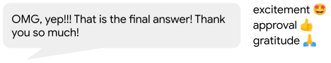 |
| This text expresses several emotions at once, including excitement, approval and gratitude. |
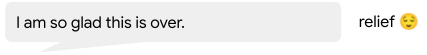 |
| This text expresses relief, a complex emotion conveying both positive and negative sentiment. |
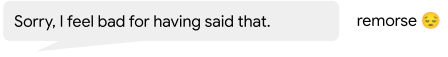 |
| This text conveys remorse, a complex emotion that is expressed frequently but is not captured by simple models of emotion. |
Building the Dataset
Our goal was to build a large dataset, focused on conversational data, where emotion is a critical component of the communication. Because the Reddit platform offers a large, publicly available volume of content that includes direct user-to-user conversation, it is a valuable resource for emotion analysis. So, we built GoEmotions using Reddit comments from 2005 (the start of Reddit) to January 2019, sourced from subreddits with at least 10k comments, excluding deleted and non-English comments.
To enable building broadly representative emotion models, we applied data curation measures to ensure the dataset does not reinforce general, nor emotion-specific, language biases. This was particularly important because Reddit has a known demographic bias leaning towards young male users, which is not reflective of a globally diverse population. The platform also introduces a skew towards toxic, offensive language. To address these concerns, we identified harmful comments using predefined terms for offensive/adult and vulgar content, and for identity and religion, which we used for data filtering and masking. We additionally filtered the data to reduce profanity, limit text length, and balance for represented emotions and sentiments. To avoid over-representation of popular subreddits and to ensure the comments also reflect less active subreddits, we also balanced the data among subreddit communities.
We created a taxonomy seeking to jointly maximize three objectives: (1) provide the greatest coverage of the emotions expressed in Reddit data; (2) provide the greatest coverage of types of emotional expressions; and (3) limit the overall number of emotions and their overlap. Such a taxonomy allows data-driven fine-grained emotion understanding, while also addressing potential data sparsity for some emotions.
Establishing the taxonomy was an iterative process to define and refine the emotion label categories. During the data labeling stages, we considered a total of 56 emotion categories. From this sample, we identified and removed emotions that were scarcely selected by raters, had low interrater agreement due to similarity to other emotions, or were difficult to detect from text. We also added emotions that were frequently suggested by raters and were well represented in the data. Finally, we refined emotion category names to maximize interpretability, leading to high interrater agreement, with 94% of examples having at least two raters agreeing on at least 1 emotion label.
The published GoEmotions dataset includes the taxonomy presented below, and was fully collected through a final round of data labeling where both the taxonomy and rating standards were pre-defined and fixed.
 |
| GoEmotions taxonomy: Includes 28 emotion categories, including “neutral”. |
<!–
| Positive | Negative | Ambiguous | ||
| admiration 👏 | joy 😃 | anger 😡 | grief 😢 | confusion 😕 |
| amusement 😂 | love ❤️ | annoyance 😒 | nervousness 😬 | curiosity 🤔 |
| approval 👍 | optimism 🤞 | disappointment | remorse 😔 | realization 💡 |
| caring 🤗 | pride 😌 | disapproval 👎 | sadness 😞 | surprise 😲 |
| desire 😍 | relief 😅 | disgust 🤮 | ||
| excitement 🤩 | embarrassment 😳 | |||
| gratitude 🙏 | fear 😨 | |||
–>
Data Analysis and Results
Emotions are not distributed uniformly in the GoEmotions dataset. Importantly, the high frequency of positive emotions reinforces our motivation for a more diverse emotion taxonomy than that offered by the canonical six basic emotions.

To validate that our taxonomic choices match the underlying data, we conduct principal preserved component analysis (PPCA), a method used to compare two datasets by extracting linear combinations of emotion judgments that exhibit the highest joint variability across two sets of raters. It therefore helps us uncover dimensions of emotion that have high agreement across raters. PPCA was used before to understand principal dimensions of emotion recognition in video and speech, and we use it here to understand the principal dimensions of emotion in text.
We find that each component is significant (with p-values < 1.5e-6 for all dimensions), indicating that each emotion captures a unique part of the data. This is not trivial, since in previous work on emotion recognition in speech, only 12 out of 30 dimensions of emotion were found to be significant.
We examine the clustering of the defined emotions based on correlations among rater judgments. With this approach, two emotions will cluster together when they are frequently co-selected by raters. We find that emotions that are related in terms of their sentiment (negative, positive and ambiguous) cluster together, despite no predefined notion of sentiment in our taxonomy, indicating the quality and consistency of the ratings. For example, if one rater chose “excitement” as a label for a given comment, it is more likely that another rater would choose a correlated sentiment, such as “joy”, rather than, say, “fear”. Perhaps surprisingly, all ambiguous emotions clustered together, and they clustered more closely with positive emotions.

Similarly, emotions that are related in terms of their intensity, such as joy and excitement, nervousness and fear, sadness and grief, annoyance and anger, are also closely correlated.

Our paper provides additional analyses and modeling experiments using GoEmotions.
Future Work: Alternatives to Human-Labeling
While GoEmotions offers a large set of human-annotated emotion data, additional emotion datasets exist that use heuristics for automatic weak-labeling. The dominant heuristic uses emotion-related Twitter tags as emotion categories, which allows one to inexpensively generate large datasets. But this approach is limited for multiple reasons: the language used on Twitter is demonstrably different than many other language domains, thus limiting the applicability of the data; tags are human generated, and, when used directly, are prone to duplication, overlap, and other taxonomic inconsistencies; and the specificity of this approach to Twitter limits its applications to other language corpora.
We propose an alternative, and more easily available heuristic in which emojis embedded in user conversation serve as a proxy for emotion categories. This approach can be applied to any language corpora containing a reasonable occurence of emojis, including many that are conversational. Because emojis are more standardized and less sparse than Twitter-tags, they present fewer inconsistencies.
Note that both of the proposed approaches — using Twitter tags and using emojis — are not directly aimed at emotion understanding, but rather at variants of conversational expression. For example, in the conversation below, 🙏 conveys gratitude, 🎂 conveys a celebratory expression, and 🎁 is a literal replacement for ‘present’. Similarly, while many emojis are associated with emotion-related expressions, emotions are subtle and multi-faceted, and in many cases no one emoji can truly capture the full complexity of an emotion. Moreover, emojis capture varying expressions beyond emotions. For these reasons, we consider them as expressions rather than emotions.

This type of data can be valuable for building expressive conversational agents, as well as for suggesting contextual emojis, and is a particularly interesting area of future work.
Conclusion
The GoEmotions dataset provides a large, manually annotated, dataset for fine-grained emotion prediction. Our analysis demonstrates the reliability of the annotations and high coverage of the emotions expressed in Reddit comments. We hope that GoEmotions will be a valuable resource to language-based emotion researchers, and will allow practitioners to build creative emotion-driven applications, addressing a wide range of user emotions.
Acknowledgements
This blog presents research done by Dora Demszky (while interning at Google), Dana Alon (previously Movshovitz-Attias), Jeongwoo Ko, Alan Cowen, Gaurav Nemade, and Sujith Ravi. We thank Peter Young for his infrastructure and open sourcing contributions. We thank Erik Vee, Ravi Kumar, Andrew Tomkins, Patrick Mcgregor, and the Learn2Compress team for support and sponsorship of this research project.


